Create gstat objects, or subset it

Function that creates gstat objects; objects that hold all the information necessary for univariate or multivariate geostatistical prediction (simple, ordinary or universal (co)kriging), or its conditional or unconditional Gaussian or indicator simulation equivalents. Multivariate gstat object can be subsetted.

Usage

gstat(g, id, formula, locations, data, model = NULL, beta,
  nmax = Inf, nmin = 0, omax = 0, maxdist = Inf, force = FALSE,
  dummy = FALSE, set, fill.all = FALSE,
  fill.cross = TRUE, variance = "identity", weights = NULL, merge, 
  degree = 0, vdist = FALSE, lambda = 1.0)
# S3 method for class 'gstat'
print(x, ...)

Arguments

g: gstat object to append to; if missing, a new gstat object is created
id: identifier of new variable; if missing, varn is used with n the number for this variable. If a cross variogram is entered, id should be a vector with the two id values , e.g. c("zn", "cd"), further only supplying arguments g and model. It is advisable not to use expressions, such as log(zinc), as identifiers, as this may lead to complications later on.
formula: formula that defines the dependent variable as a linear model of independent variables; suppose the dependent variable has name z, for ordinary and simple kriging use the formula z~1; for simple kriging also define beta (see below); for universal kriging, suppose z is linearly dependent on x and y, use the formula z~x+y
locations: formula with only independent variables that define the spatial data locations (coordinates), e.g. ~x+y; if data has a coordinates method to extract its coordinates this argument can be ignored (see package sp for classes for point or grid data).
data: data frame; contains the dependent variable, independent variables, and locations.
model: variogram model for this id; defined by a call to vgm; see argument id to see how cross variograms are entered
beta: for simple kriging (and simulation based on simple kriging): vector with the trend coefficients (including intercept); if no independent variables are defined the model only contains an intercept and this should be the expected value; for cross variogram computations: mean parameters to be used instead of the OLS estimates
nmax: for local kriging: the number of nearest observations that should be used for a kriging prediction or simulation, where nearest is defined in terms of the space of the spatial locations
nmin: for local kriging: if the number of nearest observations within distance maxdist is less than nmin, a missing value will be generated, unless force==TRUE; see maxdist
omax: maximum number of observations to select per octant (3D) or quadrant (2D); only relevant if maxdist has been defined as well
maxdist: for local kriging: only observations within a distance of maxdist from the prediction location are used for prediction or simulation; if combined with nmax, both criteria apply
force: for local kriging, force neighbourhood selection: in case nmin is given, search beyond maxdist until nmin neighbours are found. A missing value is returned if this is not possible.
dummy: logical; if TRUE, consider this data as a dummy variable (only necessary for unconditional simulation)
set: named list with optional parameters to be passed to gstat (only set commands of gstat are allowed, and not all of them may be relevant; see the manual for gstat stand-alone, URL below )
x: gstat object to print
fill.all: logical; if TRUE, fill all of the direct variogram and, depending on the value of fill.cross also all cross variogram model slots in g with the given variogram model
fill.cross: logical; if TRUE, fill all of the cross variograms, if FALSE fill only all direct variogram model slots in g with the given variogram model (only if fill.all is used)
variance: character; variance function to transform to non-stationary covariances; "identity" does not transform, other options are "mu" (Poisson) and "mu(1-mu)" (binomial)
weights: numeric vector; if present, covariates are present, and variograms are missing weights are passed to OLS prediction routines resulting in WLS; if variograms are given, weights should be 1/variance, where variance specifies location-specific measurement error; see references section below
merge: either character vector of length 2, indicating two ids that share a common mean; the more general gstat merging of any two coefficients across variables is obtained when a list is passed, with each element a character vector of length 4, in the form c("id1", 1,"id2", 2). This merges the first parameter for variable id1 to the second of variable id2.
degree: order of trend surface in the location, between 0 and 3
vdist: logical; if TRUE, instead of Euclidian distance variogram distance is used for selecting the nmax nearest neighbours, after observations within distance maxdist (Euclidian/geographic) have been pre-selected
lambda: test feature; doesn't do anything (yet)
...: arguments that are passed to the printing of variogram models only

Details

to print the full contents of the object g returned, use as.list(g) or print.default(g)

Value

an object of class gstat, which inherits from list. Its components are:

data: list; each element is a list with the formula, locations, data, nvars, beta, etc., for a variable
model: list; each element contains a variogram model; names are those of the elements of data; cross variograms have names of the pairs of data elements, separated by a . (e.g.: var1.var2

)

set: list; named list, corresponding to set name=value; gstat commands (look up the set command in the gstat manual for a full list)

References

http://www.gstat.org/ Pebesma, E.J., 2004. Multivariable geostatistics in S: the gstat package. Computers and Geosciences, 30: 683-691.

for kriging with known, varying measurement errors (weights), see e.g. Delhomme, J.P. Kriging in the hydrosciences. Advances in Water Resources, 1(5):251-266, 1978; see also the section Kriging with known measurement errors in the gstat user's manual, http://www.gstat.org/

Author

Edzer Pebesma

Note

The function currently copies the data objects into the gstat object, so this may become a large object. I would like to copy only the name of the data frame, but could not get this to work. Any help is appreciated.

Subsetting (see examples) is done using the id's of the variables, or using numeric subsets. Subsetted gstat objects only contain cross variograms if (i) the original gstat object contained them and (ii) the order of the subset indexes increases, numerically, or given the order they have in the gstat object.

The merge item may seem obscure. Still, for colocated cokriging, it is needed. See texts by Goovaerts, Wackernagel, Chiles and Delfiner, or look for standardised ordinary kriging in the 1992 Deutsch and Journel or Isaaks and Srivastava. In these cases, two variables share a common mean parameter. Gstat generalises this case: any two variables may share any of the regression coefficients; allowing for instance analysis of covariance models, when variograms were left out (see e.g. R. Christensen's “Plane answers” book on linear models). The tests directory of the package contains examples in file merge.R. There is also demo(pcb) which merges slopes across years, but with year-dependent intercept.

Examples

library(sp)
data(meuse)
coordinates(meuse) = ~x+y
# let's do some manual fitting of two direct variograms and a cross variogram
g <- gstat(id = "ln.zinc", formula = log(zinc)~1, data = meuse)
g <- gstat(g, id = "ln.lead", formula = log(lead)~1, data = meuse)
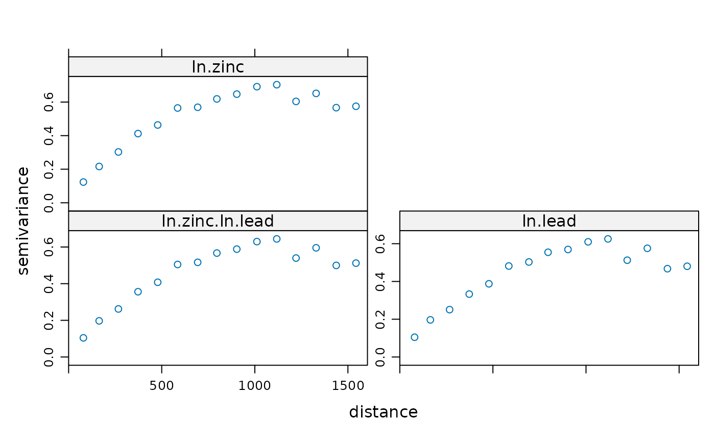
# examine variograms and cross variogram:
plot(variogram(g))

# enter direct variograms:
g <- gstat(g, id = "ln.zinc", model = vgm(.55, "Sph", 900, .05))
g <- gstat(g, id = "ln.lead", model = vgm(.55, "Sph", 900, .05))
# enter cross variogram:
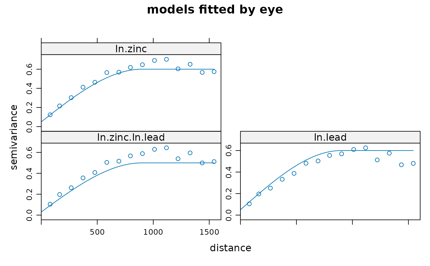
g <- gstat(g, id = c("ln.zinc", "ln.lead"), model = vgm(.47, "Sph", 900, .03))
# examine fit:
plot(variogram(g), model = g$model, main = "models fitted by eye")

# see also demo(cokriging) for a more efficient approach
g["ln.zinc"]
#> data:
#> ln.zinc : formula = log(zinc)`~`1 ; data dim = 155 x 12
#> variograms:
#>            model psill range
#> ln.zinc[1]   Nug  0.05     0
#> ln.zinc[2]   Sph  0.55   900
g["ln.lead"]
#> data:
#> ln.lead : formula = log(lead)`~`1 ; data dim = 155 x 12
#> variograms:
#>            model psill range
#> ln.lead[1]   Nug  0.05     0
#> ln.lead[2]   Sph  0.55   900
g[c("ln.zinc", "ln.lead")]
#> data:
#> ln.zinc : formula = log(zinc)`~`1 ; data dim = 155 x 12
#> ln.lead : formula = log(lead)`~`1 ; data dim = 155 x 12
#> variograms:
#>                    model psill range
#> ln.zinc[1]           Nug  0.05     0
#> ln.zinc[2]           Sph  0.55   900
#> ln.lead[1]           Nug  0.05     0
#> ln.lead[2]           Sph  0.55   900
#> ln.zinc.ln.lead[1]   Nug  0.03     0
#> ln.zinc.ln.lead[2]   Sph  0.47   900
g[1]
#> data:
#> ln.zinc : formula = log(zinc)`~`1 ; data dim = 155 x 12
#> variograms:
#>            model psill range
#> ln.zinc[1]   Nug  0.05     0
#> ln.zinc[2]   Sph  0.55   900
g[2]
#> data:
#> ln.lead : formula = log(lead)`~`1 ; data dim = 155 x 12
#> variograms:
#>            model psill range
#> ln.lead[1]   Nug  0.05     0
#> ln.lead[2]   Sph  0.55   900

# Inverse distance interpolation with inverse distance power set to .5:
# (kriging variants need a variogram model to be specified)
data(meuse.grid)
gridded(meuse.grid) = ~x+y
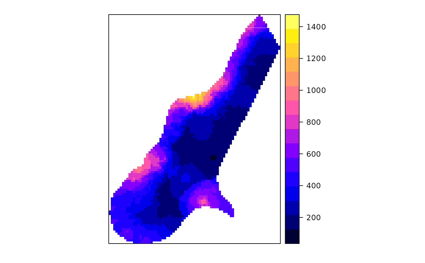
meuse.gstat <- gstat(id = "zinc", formula = zinc ~ 1, data = meuse, 
  nmax = 7, set = list(idp = .5))
meuse.gstat
#> data:
#> zinc : formula = zinc`~`1 ; data dim = 155 x 12 nmax = 7
#> set idp = 0.5; 
z <- predict(meuse.gstat, meuse.grid)
#> [inverse distance weighted interpolation]
spplot(z["zinc.pred"])

# see demo(cokriging) and demo(examples) for further examples, 
# and the manuals for predict and image

# local universal kriging
gmeuse <- gstat(id = "log_zinc", formula = log(zinc)~sqrt(dist), data = meuse)
# variogram of residuals
vmeuse.res <- fit.variogram(variogram(gmeuse), vgm(1, "Exp", 300, 1))
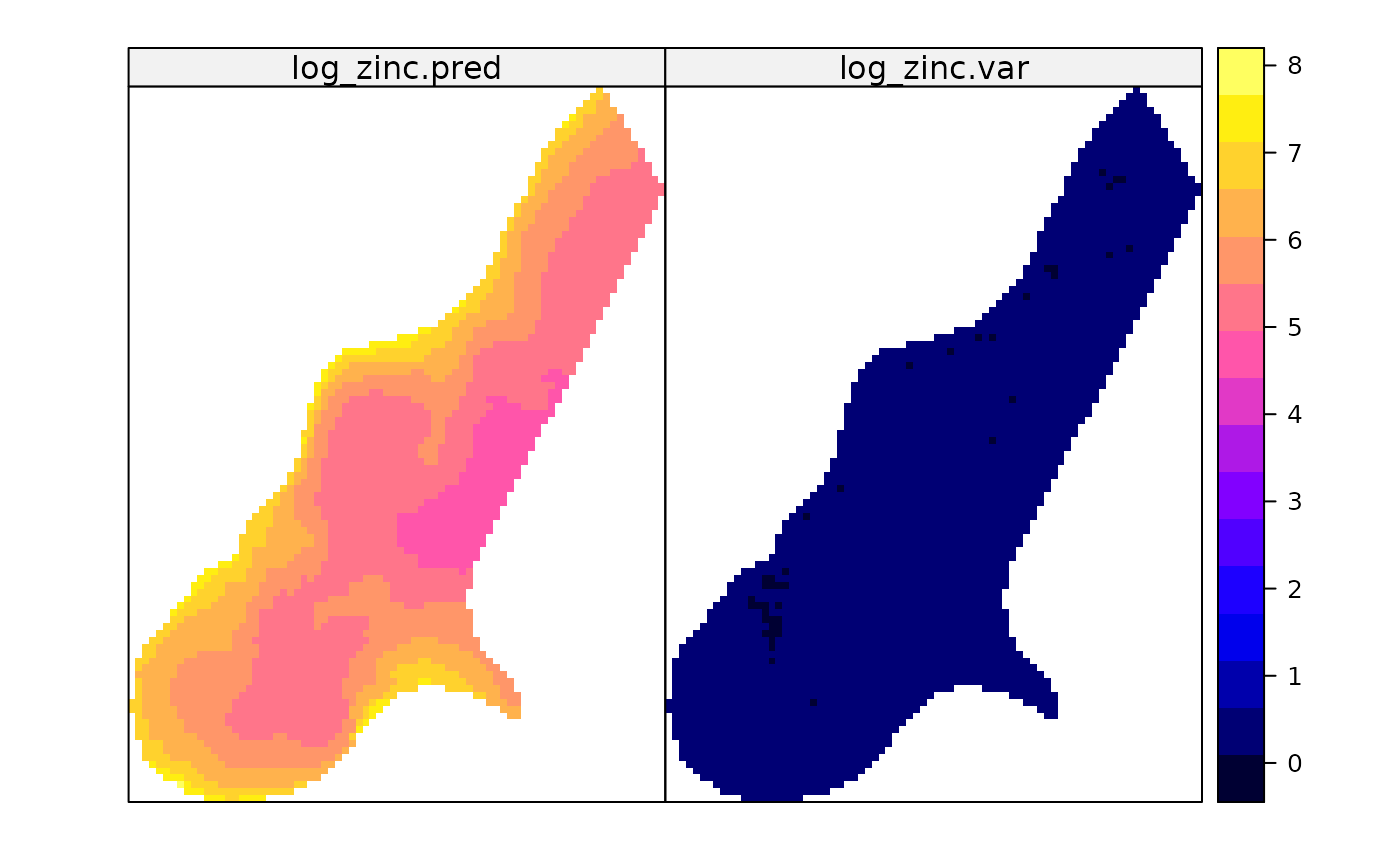
# prediction from local neighbourhoods within radius of 170 m or at least 10 points
gmeuse <- gstat(id = "log_zinc", formula = log(zinc)~sqrt(dist),
  data = meuse, maxdist=170, nmin=10, force=TRUE, model=vmeuse.res)
predmeuse <- predict(gmeuse, meuse.grid)
#> [using universal kriging]
spplot(predmeuse)