Calculate Spatio-Temporal Sample Variogram

Calculates the sample variogram from spatio-temporal data.

Usage

variogramST(formula, locations, data, ..., tlags = 0:15,  cutoff,
  width = cutoff/15, boundaries = seq(0, cutoff, width),
  progress = interactive(), pseudo = TRUE, assumeRegular = FALSE, 
  na.omit = FALSE, cores = 1)

Arguments

formula: formula, specifying the dependent variable.
locations: A STFDF or STSDF containing the variable; kept for compatibility reasons with variogram, either locations or data must be provided.
data: A STFDF, STSDF or STIDF containing the variable.
...: any other arguments that will be passed to the underlying variogram function. In case of using data of type STIDF, the argument tunit is recommended (and only used in the case of STIDF) to set the temporal unit of the tlags. Additionally, twindow can be passed to control the temporal window used for temporal distance calculations. This builds on the property of xts being ordered and only the next twindow instances are considered. This avoids the need of huge temporal distance matrices. The default uses twice the number as the average difference goes into the temporal cutoff.
tlags: integer; time lags to consider or in case data is of class STIDF the actual temporal boundaries with time unit given by tunit otherwise the same unit as diff on the index of the time slot will generate is assumed.
cutoff: spatial separation distance up to which point pairs are included in semivariance estimates; as a default, the length of the diagonal of the box spanning the data is divided by three.
width: the width of subsequent distance intervals into which data point pairs are grouped for semivariance estimates, by default the cutoff is divided into 15 equal lags.
boundaries: numerical vector with distance interval upper boundaries; values should be strictly increasing
progress: logical; if TRUE, show text progress bar
pseudo: integer; use pseudo cross variogram for computing time-lagged spatial variograms? -1: find out from coordinates – if they are equal then yes, else no; 0: no; 1: yes.
assumeRegular: logical; whether the time series should be assumed regular. The first time step is assumed to be representative for the whole series. Note, that temporal lags are considered by index, and no check is made whether pairs actually have the desired separating distance.
na.omit: shall all NA values in the spatio-temporal variogram be dropped? In case where complete rows or columns in the variogram consists of NA only, plot might produce a distorted picture.
cores: number of cores to use in parallel

Value

The spatio-temporal sample variogram contains besides the fields np, dist and gamma the spatio-temporal fields, timelag, spacelag and avgDist, the first of which indicates the time lag used, the second and third different spatial lags. spacelag is the midpoint in the spatial lag intervals as passed by the parameter boundaries, whereas avgDist is the average distance between the point pairs found in a distance interval over all temporal lags (i.e. the averages of the values dist per temporal lag.) To compute variograms for space lag \(h\) and time lag \(t\), the pseudo cross variogram \((Z_i(s)-Z_{i+t}(s+h))^2\) is averaged over all time lagged observation sets \(Z_i\) and \(Z_{i+t}\) available (weighted by the number of pairs involved).

References

Cressie, N.A.C., 1993, Statistics for Spatial Data, Wiley.

Cressie, N., C. Wikle, 2011, Statistics for Spatio-temporal Data, Wiley.

http://www.gstat.org/

Pebesma, E.J., 2004. Multivariable geostatistics in S: the gstat package. Computers and Geosciences, 30: 683-691.

Author

Edzer Pebesma, Benedikt Graeler

Examples

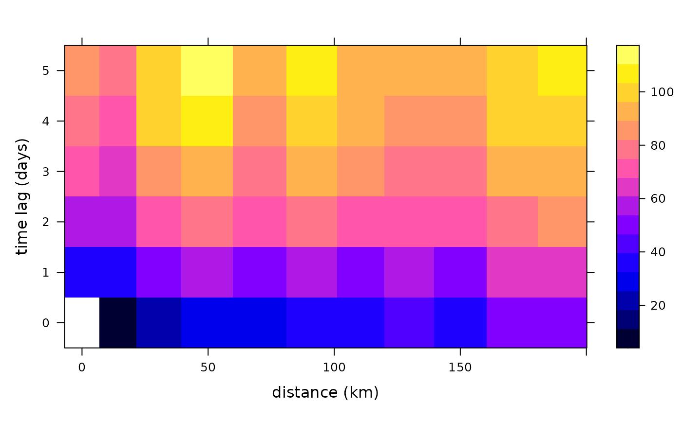
# The following spatio-temporal variogram has been calcualted through
# vv = variogram(PM10~1, r5to10, width=20, cutoff = 200, tlags=0:5)
# in the vignette "st".

data(vv)
str(vv)
#> Classes ‘StVariogram’ and 'data.frame':	66 obs. of  7 variables:
#>  $ np      : num  0 3456 16554 21257 33547 ...
#>  $ dist    : num  NA 13.8 29.5 49.1 70.4 ...
#>  $ gamma   : num  NA 11 23.4 29.6 31.2 ...
#>  $ id      : chr  "lag0" "lag0" "lag0" "lag0" ...
#>  $ timelag : num  0 0 0 0 0 0 0 0 0 0 ...
#>   ..- attr(*, "units")= chr "days"
#>  $ spacelag: num  0 10 30 50 70 90 110 130 150 170 ...
#>   ..- attr(*, "units")= chr "km"
#>  $ avgDist : num  0 13.8 29.5 49.1 70.4 ...
#>  - attr(*, "boundaries")= num [1:11] 0 20 40 60 80 100 120 140 160 180 ...
plot(vv)