TransGaussian kriging using Box-Cox transforms

TransGaussian (ordinary) kriging function using Box-Cox transforms

Usage

krigeTg(formula, locations, newdata, model = NULL, ...,
  nmax = Inf, nmin = 0, maxdist = Inf, block = numeric(0),
  nsim = 0, na.action = na.pass, debug.level = 1,
  lambda = 1.0)

Arguments

formula: formula that defines the dependent variable as a linear model of independent variables; suppose the dependent variable has name z, for ordinary and use a formula like z~1; the dependent variable should be NOT transformed.
locations: object of class Spatial, with observations
newdata: Spatial object with prediction/simulation locations; the coordinates should have names as defined in locations
model: variogram model of the TRANSFORMED dependent variable, see vgm, or fit.variogram
nmax: for local kriging: the number of nearest observations that should be used for a kriging prediction or simulation, where nearest is defined in terms of the space of the spatial locations. By default, all observations are used
nmin: for local kriging: if the number of nearest observations within distance maxdist is less than nmin, a missing value will be generated; see maxdist
maxdist: for local kriging: only observations within a distance of maxdist from the prediction location are used for prediction or simulation; if combined with nmax, both criteria apply
block: does not function correctly, afaik
nsim: does not function correctly, afaik
na.action: function determining what should be done with missing values in 'newdata'. The default is to predict 'NA'. Missing values in coordinates and predictors are both dealt with.
lambda: value for the Box-Cox transform
debug.level: debug level, passed to predict; use -1 to see progress in percentage, and 0 to suppress all printed information
...: other arguments that will be passed to gstat

Details

Function krigeTg uses transGaussian kriging as explained in https://www.math.umd.edu/~bnk/bak/Splus/kriging.html.

As it uses the R/gstat krige function to derive everything, it needs in addition to ordinary kriging on the transformed scale a simple kriging step to find m from the difference between the OK and SK prediction variance, and a kriging/BLUE estimation step to obtain the estimate of \(\mu\).

For further details, see krige and predict.

Value

an SpatialPointsDataFrame object containing the fields: m for the m (Lagrange) parameter for each location; var1SK.pred the \(c_0 C^{-1}\) correction obtained by muhat for the mean estimate at each location; var1SK.var the simple kriging variance; var1.pred the OK prediction on the transformed scale; var1.var the OK kriging variance on the transformed scale; var1TG.pred the transGaussian kriging predictor; var1TG.var the transGaussian kriging variance, obtained by \(\phi'(\hat{\mu},\lambda)^2 \sigma^2_{OK}\)

References

N.A.C. Cressie, 1993, Statistics for Spatial Data, Wiley.

http://www.gstat.org/

Author

Edzer Pebesma

Examples

# \donttest{
library(sp)
data(meuse)
coordinates(meuse) = ~x+y
data(meuse.grid)
gridded(meuse.grid) = ~x+y
v = vgm(1, "Exp", 300)
x1 = krigeTg(zinc~1,meuse,meuse.grid,v, lambda=1) # no transform
#> [using ordinary kriging]
#> [generalized least squares trend estimation]
#> [using simple kriging]
x2 = krige(zinc~1,meuse,meuse.grid,v)
#> [using ordinary kriging]
summary(x2$var1.var-x1$var1TG.var)
#>    Min. 1st Qu.  Median    Mean 3rd Qu.    Max. 
#>       0       0       0       0       0       0 
summary(x2$var1.pred-x1$var1TG.pred)
#>       Min.    1st Qu.     Median       Mean    3rd Qu.       Max. 
#> -2.274e-13 -5.684e-14  0.000e+00 -8.573e-15  0.000e+00  4.547e-13 
lambda = -0.25
m = fit.variogram(variogram((zinc^lambda-1)/lambda ~ 1,meuse), vgm(1, "Exp", 300))
x = krigeTg(zinc~1,meuse,meuse.grid,m,lambda=-.25)
#> [using ordinary kriging]
#> [generalized least squares trend estimation]
#> [using simple kriging]
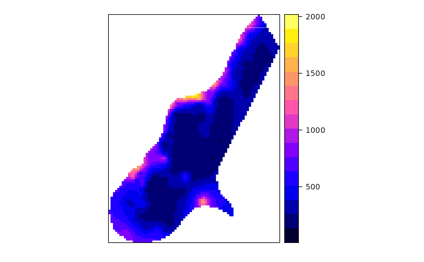
spplot(x["var1TG.pred"], col.regions=bpy.colors())

summary(meuse$zinc)
#>    Min. 1st Qu.  Median    Mean 3rd Qu.    Max. 
#>   113.0   198.0   326.0   469.7   674.5  1839.0 
summary(x$var1TG.pred)
#>    Min. 1st Qu.  Median    Mean 3rd Qu.    Max. 
#>   130.7   229.7   299.5   403.2   521.3  1894.3 
# }