Spatial simultaneous autoregressive error model estimation by GMM

An implementation of Kelejian and Prucha's generalised moments estimator for the autoregressive parameter in a spatial model.

Usage

GMerrorsar(formula, data = list(), listw, na.action = na.fail,
 zero.policy = attr(listw, "zero.policy"), method="nlminb", arnoldWied=FALSE, 
 control = list(), pars, scaleU=FALSE, verbose=NULL, legacy=FALSE,
 se.lambda=TRUE, returnHcov=FALSE, pWOrder=250, tol.Hcov=1.0e-10)
# S3 method for class 'Gmsar'
summary(object, correlation = FALSE, Hausman=FALSE, ...)
GMargminImage(obj, lambdaseq, s2seq)

Arguments

formula: a symbolic description of the model to be fit. The details of model specification are given for lm()
data: an optional data frame containing the variables in the model. By default the variables are taken from the environment which the function is called.
listw: a listw object created for example by nb2listw
na.action: a function (default na.fail), can also be na.omit or na.exclude with consequences for residuals and fitted values - in these cases the weights list will be subsetted to remove NAs in the data. It may be necessary to set zero.policy to TRUE because this subsetting may create no-neighbour observations. Note that only weights lists created without using the glist argument to nb2listw may be subsetted.
zero.policy: default NULL, use global option value; if TRUE assign zero to the lagged value of zones without neighbours, if FALSE (default) assign NA - causing GMerrorsar() to terminate with an error
method: default "nlminb", or optionally a method passed to optim to use an alternative optimizer
arnoldWied: default FALSE
control: A list of control parameters. See details in optim or nlminb.
pars: starting values for \(\lambda\) and \(\sigma^2\) for GMM optimisation, if missing (default), approximated from initial OLS model as the autocorrelation coefficient corrected for weights style and model sigma squared
scaleU: Default FALSE: scale the OLS residuals before computing the moment matrices; only used if the pars argument is missing
verbose: default NULL, use global option value; if TRUE, reports function values during optimization.
legacy: default FALSE - compute using the unfiltered values of the response and right hand side variables; if TRUE - compute the fitted value and residuals from the spatially filtered model using the spatial error parameter
se.lambda: default TRUE, use the analytical method described in http://econweb.umd.edu/~prucha/STATPROG/OLS/desols.pdf
returnHcov: default FALSE, return the Vo matrix for a spatial Hausman test
tol.Hcov: the tolerance for computing the Vo matrix (default=1.0e-10)
pWOrder: default 250, if returnHcov=TRUE, pass this order to powerWeights as the power series maximum limit
object, obj: Gmsar object from GMerrorsar
correlation: logical; (default=FALSE), TRUE not available
Hausman: if TRUE, the results of the Hausman test for error models are reported
...: summary arguments passed through
lambdaseq: if given, an increasing sequence of lambda values for gridding
s2seq: if given, an increasing sequence of sigma squared values for gridding

Details

When the control list is set with care, the function will converge to values close to the ML estimator without requiring computation of the Jacobian, the most resource-intensive part of ML estimation.

Note that the fitted() function for the output object assumes that the response variable may be reconstructed as the sum of the trend, the signal, and the noise (residuals). Since the values of the response variable are known, their spatial lags are used to calculate signal components (Cressie 1993, p. 564). This differs from other software, including GeoDa, which does not use knowledge of the response variable in making predictions for the fitting data.

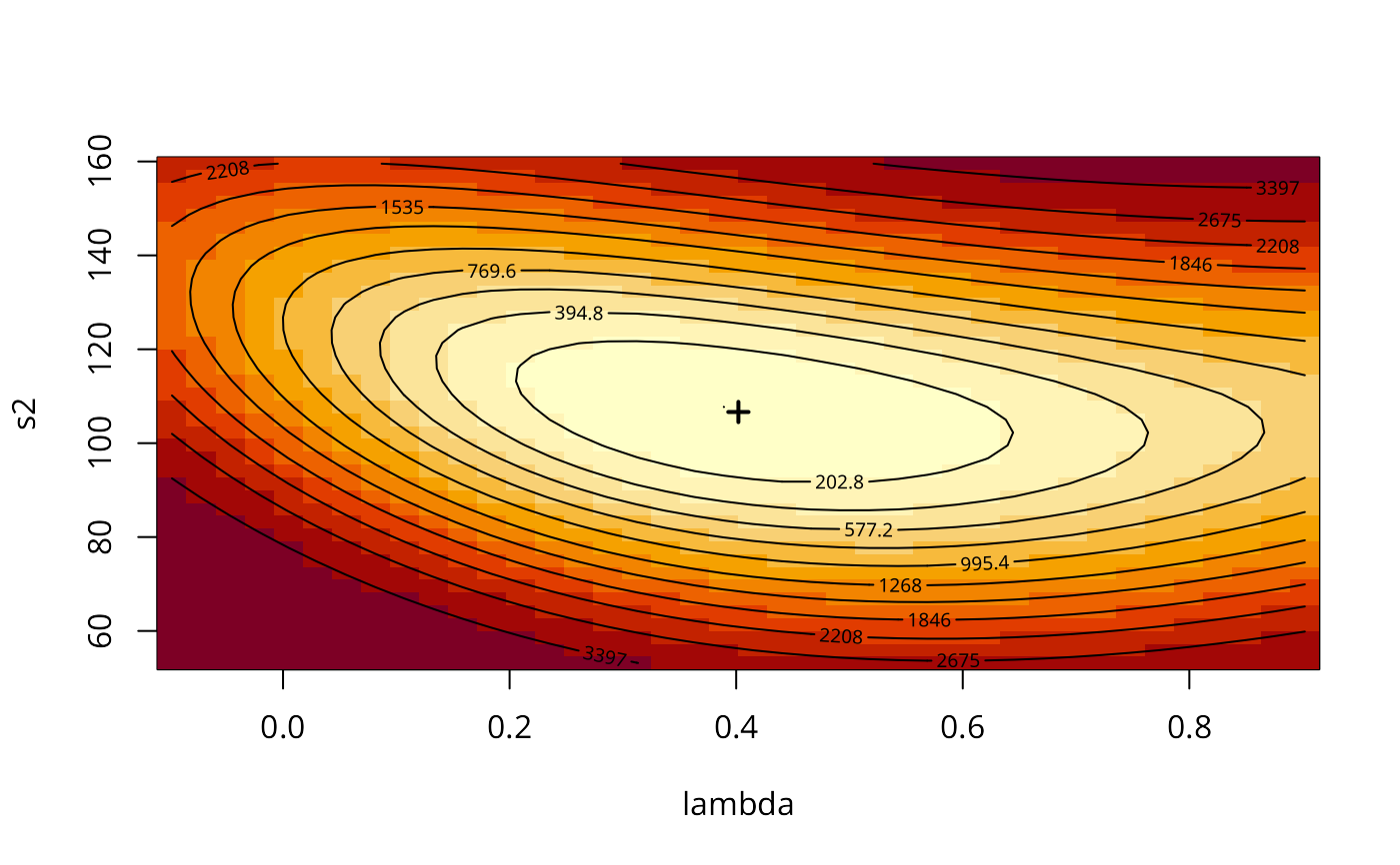
The GMargminImage may be used to visualize the shape of the surface of the argmin function used to find lambda.

Value

A list object of class Gmsar

type: "ERROR"
lambda: simultaneous autoregressive error coefficient
coefficients: GMM coefficient estimates
rest.se: GMM coefficient standard errors
s2: GMM residual variance
SSE: sum of squared GMM errors
parameters: number of parameters estimated
lm.model: the lm object returned when estimating for \(\lambda=0\)
call: the call used to create this object
residuals: GMM residuals
lm.target: the lm object returned for the GMM fit
fitted.values: Difference between residuals and response variable
formula: model formula
aliased: if not NULL, details of aliased variables
zero.policy: zero.policy for this model
vv: list of internal bigG and litg components for testing optimisation surface
optres: object returned by optimizer
pars: start parameter values for optimisation
Hcov: Spatial DGP covariance matrix for Hausman test if available
legacy: input choice of unfiltered or filtered values
lambda.se: value computed if input argument TRUE
arnoldWied: were Arnold-Wied moments used
GMs2: GM argmin sigma squared
scaleU: input choice of scaled OLS residuals
vcov: variance-covariance matrix of regression coefficients
na.action: (possibly) named vector of excluded or omitted observations if non-default na.action argument used

References

Kelejian, H. H., and Prucha, I. R., 1999. A Generalized Moments Estimator for the Autoregressive Parameter in a Spatial Model. International Economic Review, 40, pp. 509–533; Cressie, N. A. C. 1993 Statistics for spatial data, Wiley, New York.

Roger Bivand, Gianfranco Piras (2015). Comparing Implementations of Estimation Methods for Spatial Econometrics. Journal of Statistical Software, 63(18), 1-36. doi:10.18637/jss.v063.i18 .

Author

Luc Anselin and Roger Bivand

Examples

#require("spdep", quietly=TRUE)
data(oldcol, package="spdep")
COL.errW.eig <- errorsarlm(CRIME ~ INC + HOVAL, data=COL.OLD,
 spdep::nb2listw(COL.nb, style="W"), method="eigen")
(x <- summary(COL.errW.eig, Hausman=TRUE))
#> 
#> Call:
#> errorsarlm(formula = CRIME ~ INC + HOVAL, data = COL.OLD, listw = spdep::nb2listw(COL.nb, 
#>     style = "W"), method = "eigen")
#> 
#> Residuals:
#>       Min        1Q    Median        3Q       Max 
#> -34.81174  -6.44031  -0.72142   7.61476  23.33626 
#> 
#> Type: error 
#> Coefficients: (asymptotic standard errors) 
#>              Estimate Std. Error z value  Pr(>|z|)
#> (Intercept) 59.893219   5.366163 11.1613 < 2.2e-16
#> INC         -0.941312   0.330569 -2.8476 0.0044057
#> HOVAL       -0.302250   0.090476 -3.3407 0.0008358
#> 
#> Lambda: 0.56179, LR test value: 7.9935, p-value: 0.0046945
#> Asymptotic standard error: 0.13387
#>     z-value: 4.1966, p-value: 2.7098e-05
#> Wald statistic: 17.611, p-value: 2.7098e-05
#> 
#> Log likelihood: -183.3805 for error model
#> ML residual variance (sigma squared): 95.575, (sigma: 9.7762)
#> Number of observations: 49 
#> Number of parameters estimated: 5 
#> AIC: 376.76, (AIC for lm: 382.75)
#> Hausman test: 4.902, df: 3, p-value: 0.17911
#> 
coef(x)
#>               Estimate Std. Error   z value     Pr(>|z|)
#> (Intercept) 59.8932190 5.36616256 11.161276 0.0000000000
#> INC         -0.9413120 0.33056857 -2.847554 0.0044056574
#> HOVAL       -0.3022502 0.09047605 -3.340665 0.0008357787
COL.errW.GM <- GMerrorsar(CRIME ~ INC + HOVAL, data=COL.OLD,
 spdep::nb2listw(COL.nb, style="W"), returnHcov=TRUE)
(x <- summary(COL.errW.GM, Hausman=TRUE))
#> 
#> Call:
#> GMerrorsar(formula = CRIME ~ INC + HOVAL, data = COL.OLD, listw = spdep::nb2listw(COL.nb, 
#>     style = "W"), returnHcov = TRUE)
#> 
#> Residuals:
#>      Min       1Q   Median       3Q      Max 
#> -30.5432  -6.5553  -2.1921  10.0553  28.7497 
#> 
#> Type: GM SAR estimator
#> Coefficients: (GM standard errors) 
#>              Estimate Std. Error z value  Pr(>|z|)
#> (Intercept) 62.513752   5.121339  12.207 < 2.2e-16
#> INC         -1.128283   0.339745  -3.321  0.000897
#> HOVAL       -0.296957   0.095699  -3.103  0.001915
#> 
#> Lambda: 0.40196 (standard error): 0.42334 (z-value): 0.94948
#> Residual variance (sigma squared): 106.64, (sigma: 10.327)
#> GM argmin sigma squared: 106.36
#> Number of observations: 49 
#> Number of parameters estimated: 5 
#> Hausman test: 6.6406, df: 3, p-value: 0.08428
#> 
coef(x)
#>               Estimate Std. Error   z value     Pr(>|z|)
#> (Intercept) 62.5137525 5.12133863 12.206526 0.0000000000
#> INC         -1.1282834 0.33974492 -3.320972 0.0008970455
#> HOVAL       -0.2969573 0.09569889 -3.103038 0.0019154486
aa <- GMargminImage(COL.errW.GM)
levs <- quantile(aa$z, seq(0, 1, 1/12))
image(aa, breaks=levs, xlab="lambda", ylab="s2")
points(COL.errW.GM$lambda, COL.errW.GM$s2, pch=3, lwd=2)
contour(aa, levels=signif(levs, 4), add=TRUE)

COL.errW.GM1 <- GMerrorsar(CRIME ~ INC + HOVAL, data=COL.OLD,
 spdep::nb2listw(COL.nb, style="W"))
summary(COL.errW.GM1)
#> 
#> Call:
#> GMerrorsar(formula = CRIME ~ INC + HOVAL, data = COL.OLD, listw = spdep::nb2listw(COL.nb, 
#>     style = "W"))
#> 
#> Residuals:
#>      Min       1Q   Median       3Q      Max 
#> -30.5432  -6.5553  -2.1921  10.0553  28.7497 
#> 
#> Type: GM SAR estimator
#> Coefficients: (GM standard errors) 
#>              Estimate Std. Error z value  Pr(>|z|)
#> (Intercept) 62.513752   5.121339  12.207 < 2.2e-16
#> INC         -1.128283   0.339745  -3.321  0.000897
#> HOVAL       -0.296957   0.095699  -3.103  0.001915
#> 
#> Lambda: 0.40196 (standard error): 0.42334 (z-value): 0.94948
#> Residual variance (sigma squared): 106.64, (sigma: 10.327)
#> GM argmin sigma squared: 106.36
#> Number of observations: 49 
#> Number of parameters estimated: 5 
#> 
require("sf", quietly=TRUE)
nydata <- st_read(system.file("shapes/NY8_bna_utm18.gpkg", package="spData")[1], quiet=TRUE)
suppressMessages(nyadjmat <- as.matrix(foreign::read.dbf(system.file(
 "misc/nyadjwts.dbf", package="spData")[1])[-1]))
suppressMessages(ID <- as.character(names(foreign::read.dbf(system.file(
 "misc/nyadjwts.dbf", package="spData")[1]))[-1]))
identical(substring(ID, 2, 10), substring(as.character(nydata$AREAKEY), 2, 10))
#> [1] TRUE
listw_NY <- spdep::mat2listw(nyadjmat, as.character(nydata$AREAKEY), style="B")
esar1f <- spautolm(Z ~ PEXPOSURE + PCTAGE65P + PCTOWNHOME, data=nydata,
 listw=listw_NY, family="SAR", method="eigen")
summary(esar1f)
#> 
#> Call: 
#> spautolm(formula = Z ~ PEXPOSURE + PCTAGE65P + PCTOWNHOME, data = nydata, 
#>     listw = listw_NY, family = "SAR", method = "eigen")
#> 
#> Residuals:
#>      Min       1Q   Median       3Q      Max 
#> -1.56754 -0.38239 -0.02643  0.33109  4.01219 
#> 
#> Coefficients: 
#>              Estimate Std. Error z value  Pr(>|z|)
#> (Intercept) -0.618193   0.176784 -3.4969 0.0004707
#> PEXPOSURE    0.071014   0.042051  1.6888 0.0912635
#> PCTAGE65P    3.754200   0.624722  6.0094 1.862e-09
#> PCTOWNHOME  -0.419890   0.191329 -2.1946 0.0281930
#> 
#> Lambda: 0.040487 LR test value: 5.2438 p-value: 0.022026 
#> Numerical Hessian standard error of lambda: 0.017201 
#> 
#> Log likelihood: -276.1069 
#> ML residual variance (sigma squared): 0.41388, (sigma: 0.64333)
#> Number of observations: 281 
#> Number of parameters estimated: 6 
#> AIC: 564.21
#> 
esar1gm <- GMerrorsar(Z ~ PEXPOSURE + PCTAGE65P + PCTOWNHOME,
 data=nydata, listw=listw_NY)
summary(esar1gm)
#> 
#> Call:GMerrorsar(formula = Z ~ PEXPOSURE + PCTAGE65P + PCTOWNHOME, 
#>     data = nydata, listw = listw_NY)
#> 
#> Residuals:
#>       Min        1Q    Median        3Q       Max 
#> -1.641411 -0.396370 -0.026618  0.341740  4.204264 
#> 
#> Type: GM SAR estimator
#> Coefficients: (GM standard errors) 
#>              Estimate Std. Error z value  Pr(>|z|)
#> (Intercept) -0.604364   0.174576 -3.4619 0.0005364
#> PEXPOSURE    0.067902   0.041164  1.6496 0.0990337
#> PCTAGE65P    3.775308   0.622965  6.0602 1.359e-09
#> PCTOWNHOME  -0.437545   0.188906 -2.3162 0.0205468
#> 
#> Lambda: 0.03605 (standard error): 0.2022 (z-value): 0.17829
#> Residual variance (sigma squared): 0.41585, (sigma: 0.64487)
#> GM argmin sigma squared: 0.45141
#> Number of observations: 281 
#> Number of parameters estimated: 6 
#> 
esar1gm1 <- GMerrorsar(Z ~ PEXPOSURE + PCTAGE65P + PCTOWNHOME,
 data=nydata, listw=listw_NY, method="Nelder-Mead")
summary(esar1gm1)
#> 
#> Call:GMerrorsar(formula = Z ~ PEXPOSURE + PCTAGE65P + PCTOWNHOME, 
#>     data = nydata, listw = listw_NY, method = "Nelder-Mead")
#> 
#> Residuals:
#>       Min        1Q    Median        3Q       Max 
#> -1.641390 -0.396374 -0.026616  0.341745  4.204277 
#> 
#> Type: GM SAR estimator
#> Coefficients: (GM standard errors) 
#>              Estimate Std. Error z value  Pr(>|z|)
#> (Intercept) -0.604384   0.174580 -3.4619 0.0005363
#> PEXPOSURE    0.067907   0.041165  1.6496 0.0990225
#> PCTAGE65P    3.775275   0.622969  6.0601  1.36e-09
#> PCTOWNHOME  -0.437518   0.188910 -2.3160 0.0205572
#> 
#> Lambda: 0.036057 (standard error): 0.20221 (z-value): 0.17832
#> Residual variance (sigma squared): 0.41585, (sigma: 0.64487)
#> GM argmin sigma squared: 0.45139
#> Number of observations: 281 
#> Number of parameters estimated: 6 
#>