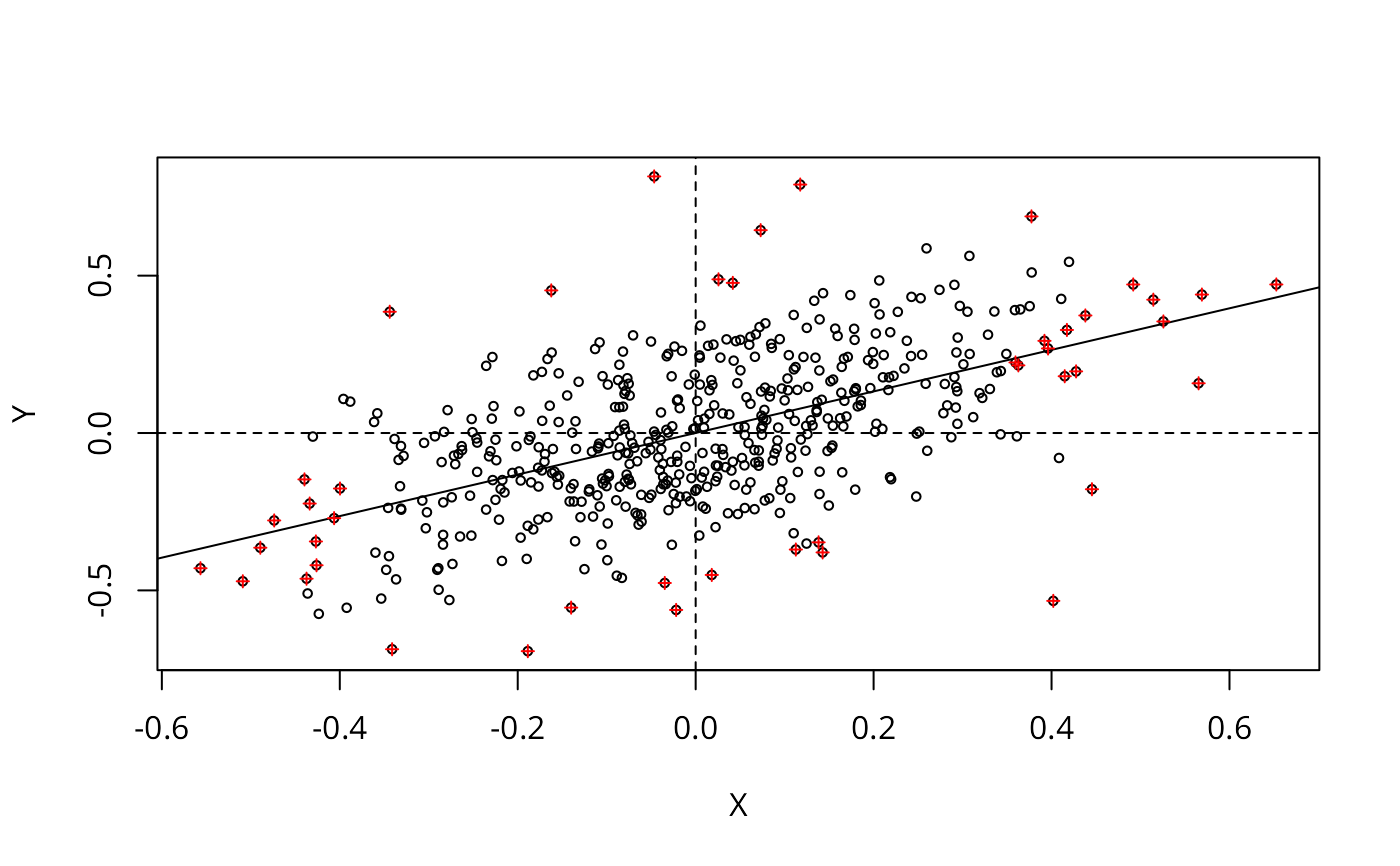
Approximate profile-likelihood estimator (APLE) scatterplot

A scatterplot decomposition of the approximate profile-likelihood estimator, and a local APLE based on the list of vectors returned by the scatterplot function.

Usage

aple.plot(x, listw, override_similarity_check=FALSE, useTrace=TRUE, do.plot=TRUE, ...)
localAple(x, listw, override_similarity_check=FALSE, useTrace=TRUE)

Arguments

x: a zero-mean detrended continuous variable
listw: a listw object from for example spdep::nb2listw
override_similarity_check: default FALSE, if TRUE - typically for row-standardised weights with asymmetric underlying general weights - similarity is not checked
useTrace: default TRUE, use trace of sparse matrix W %*% W (Li et al. (2010)), if FALSE, use crossproduct of eigenvalues of W as in Li et al. (2007)
do.plot: default TRUE: should a scatterplot be drawn
...: other arguments to be passed to plot

Details

The function solves a secondary eigenproblem of size n internally, so constructing the values for the scatterplot is quite compute and memory intensive, and is not suitable for very large n.

Value

aple.plot returns list with components:

X: A vector as described in Li et al. (2007), p. 366.
Y: A vector as described in Li et al. (2007), p. 367.

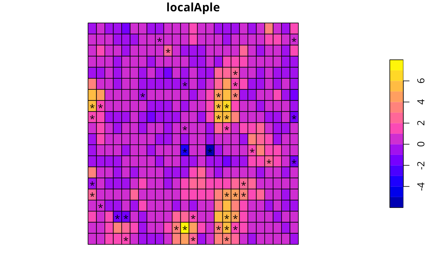
localAple returns a vector of local APLE values.

References

Li, H, Calder, C. A. and Cressie N. A. C. (2007) Beyond Moran's I: testing for spatial dependence based on the spatial autoregressive model. Geographical Analysis 39, pp. 357-375; Li, H, Calder, C. A. and Cressie N. A. C. (2012) One-step estimation of spatial dependence parameters: Properties and extensions of the APLE statistic, Journal of Multivariate Analysis 105, 68-84.

Author

Roger Bivand Roger.Bivand@nhh.no

Examples

if (FALSE) { # \dontrun{
wheat <- st_read(system.file("shapes/wheat.gpkg", package="spData")[1], quiet=TRUE)
nbr1 <- spdep::poly2nb(wheat, queen=FALSE)
nbrl <- spdep::nblag(nbr1, 2)
nbr12 <- spdep::nblag_cumul(nbrl)
cms0 <- with(as.data.frame(wheat), tapply(yield, c, median))
cms1 <- c(model.matrix(~ factor(c) -1, data=wheat) %*% cms0)
wheat$yield_detrend <- wheat$yield - cms1
plt_out <- aple.plot(as.vector(scale(wheat$yield_detrend, scale=FALSE)),
 spdep::nb2listw(nbr12, style="W"), cex=0.6)
lm_obj <- lm(Y ~ X, plt_out)
abline(lm_obj)
abline(v=0, h=0, lty=2)
zz <- summary(influence.measures(lm_obj))
infl <- as.integer(rownames(zz))
points(plt_out$X[infl], plt_out$Y[infl], pch=3, cex=0.6, col="red")
crossprod(plt_out$Y, plt_out$X)/crossprod(plt_out$X)
wheat$localAple <- localAple(as.vector(scale(wheat$yield_detrend, scale=FALSE)),
 spdep::nb2listw(nbr12, style="W"))
mean(wheat$localAple)
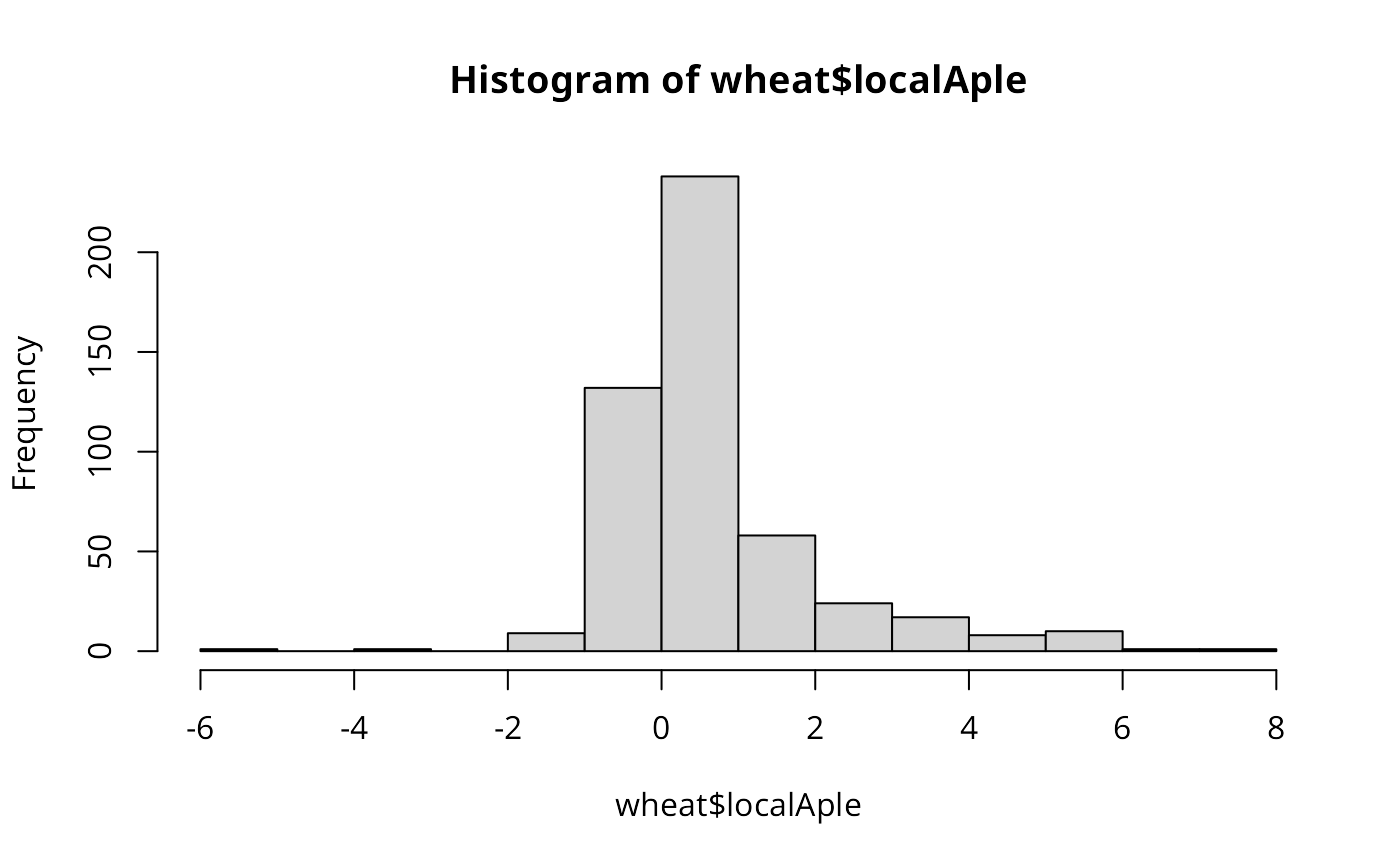
hist(wheat$localAple)
opar <- par(no.readonly=TRUE)
plot(wheat[,"localAple"], reset=FALSE)
text(st_coordinates(st_centroid(st_geometry(wheat)))[infl,], labels=rep("*", length(infl)))
par(opar)
} # }