Construct neighbours list from polygon list

The function builds a neighbours list based on regions with contiguous boundaries, that is sharing one or more boundary point. The current function is in part interpreted and may run slowly for many regions or detailed boundaries, but from 0.2-16 should not fail because of lack of memory when single polygons are built of very many border coordinates.

Usage

poly2nb(pl, row.names = NULL, snap=NULL, queen=TRUE, useC=TRUE, foundInBox=NULL)

Arguments

pl: list of polygons of class extending SpatialPolygons, or an sf or sfc object containing non-empty (multi-)polygon objects
row.names: character vector of region ids to be added to the neighbours list as attribute region.id, default seq(1, nrow(x)); if pl has row.names, they are used instead of the default sequence.
snap: boundary points less than snap distance apart are considered to indicate contiguity; used both to find candidate and actual neighbours for planar geometries, but only actual neighbours for spherical geometries, as spherical spatial indexing itself injects some fuzzyness. If not set, for all SpatialPolygons objects, the default is as before sqrt(.Machine$double.eps), with this value also used for sf objects with no coordinate reference system. For sf objects with a defined coordinate reference system, the default value is 1e-7 for geographical coordinates (approximately 10mm), is 10mm where projected coordinates are in metre units, and is converted from 10mm to the same distance in the units of the coordinates. Should the conversion fail, snap reverts to sqrt(.Machine$double.eps).
queen: if TRUE, a single shared boundary point meets the contiguity condition, if FALSE, more than one shared point is required; note that more than one shared boundary point does not necessarily mean a shared boundary line
useC: default TRUE, doing the work loop in C, may be set to false to revert to R code calling two C functions in an n*k work loop, where k is the average number of candidate neighbours
foundInBox: default NULL using R code or st_intersects() to generate candidate neighbours (using snap= if the geometries are not spherical); if not NULL (for legacy purposes) a list of length (n-1) with integer vectors of candidate neighbours (j > i) (as created by the poly_findInBoxGEOS function in rgeos for clean polygons)

Value

A neighbours list with class nb. See card for details of “nb” objects.

Note

From 0.5-8, the function includes faster bounding box indexing and other improvements contributed by Micah Altman. If a cluster is provided using set.ClusterOption, it will be used for finding candidate bounding box overlaps for exact testing for contiguity.

Until 1.1-7, sf polygons included both start and end points, so could erroneously report queen neighbourhood where only rook was present, see https://github.com/r-spatial/spdep/issues/50.

From 1.1-9 with sf 1.0-0, s2 is used in bounding box indexing internally when pl is in geographical coordinates. Because the topology engine of s2 differs from the use of GEOS for planar coordinates by sf, some output differences may be expected. Since treating spherical geometries as planar is also questionable, it is not clear whether spherical contiguous polygon neighbours should simply follow neighbours found by treating the geometries as planar https://github.com/r-spatial/s2/issues/125#issuecomment-864403372. However, current advice is not necessarily to use s2 for finding contiguity neighbours, or at least to check output.

Author

Roger Bivand Roger.Bivand@nhh.no with contributions from Micah Altman

Examples

columbus <- st_read(system.file("shapes/columbus.gpkg", package="spData")[1], quiet=TRUE)
col.gal.nb <- read.gal(system.file("weights/columbus.gal", package="spData")[1])
coords <- st_coordinates(st_centroid(st_geometry(columbus)))
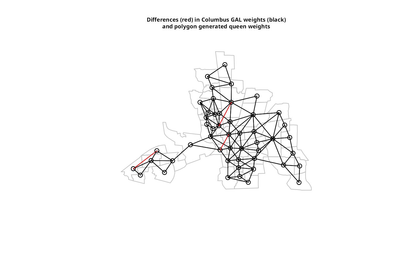
xx <- poly2nb(as(columbus, "Spatial"))
dxx <- diffnb(xx, col.gal.nb)
#> Warning: neighbour object has 46 sub-graphs
plot(st_geometry(columbus), border="grey")
plot(col.gal.nb, coords, add=TRUE)
plot(dxx, coords, add=TRUE, col="red")
title(main=paste("Differences (red) in Columbus GAL weights (black)",
 "and polygon generated queen weights", sep="\n"), cex.main=0.6)

# poly2nb with sf sfc_MULTIPOLYGON objects
sf_xx <- poly2nb(columbus)
diffnb(sf_xx, xx)
#> Warning: neighbour object has 49 sub-graphs
#> Neighbour list object:
#> Number of regions: 49 
#> Number of nonzero links: 0 
#> Percentage nonzero weights: 0 
#> Average number of links: 0 
#> 49 regions with no links:
#> 1, 2, 3, 4, 5, 6, 7, 8, 9, 10, 11, 12, 13, 14, 15, 16, 17, 18, 19, 20,
#> 21, 22, 23, 24, 25, 26, 27, 28, 29, 30, 31, 32, 33, 34, 35, 36, 37, 38,
#> 39, 40, 41, 42, 43, 44, 45, 46, 47, 48, 49
#> 49 disjoint connected subgraphs
sfc_xx <- poly2nb(st_geometry(columbus))
diffnb(sfc_xx, xx)
#> Warning: neighbour object has 49 sub-graphs
#> Neighbour list object:
#> Number of regions: 49 
#> Number of nonzero links: 0 
#> Percentage nonzero weights: 0 
#> Average number of links: 0 
#> 49 regions with no links:
#> 1, 2, 3, 4, 5, 6, 7, 8, 9, 10, 11, 12, 13, 14, 15, 16, 17, 18, 19, 20,
#> 21, 22, 23, 24, 25, 26, 27, 28, 29, 30, 31, 32, 33, 34, 35, 36, 37, 38,
#> 39, 40, 41, 42, 43, 44, 45, 46, 47, 48, 49
#> 49 disjoint connected subgraphs
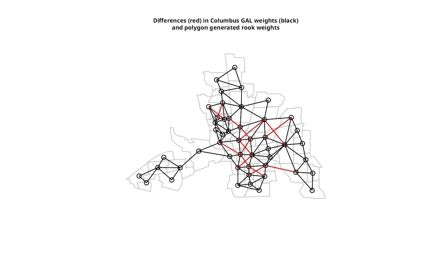
xxx <- poly2nb(as(columbus, "Spatial"), queen=FALSE)
dxxx <- diffnb(xxx, col.gal.nb)
#> Warning: neighbour object has 34 sub-graphs
plot(st_geometry(columbus), border = "grey")
plot(col.gal.nb, coords, add = TRUE)
plot(dxxx, coords, add = TRUE, col = "red")
title(main=paste("Differences (red) in Columbus GAL weights (black)",
 "and polygon generated rook weights", sep="\n"), cex.main=0.6)

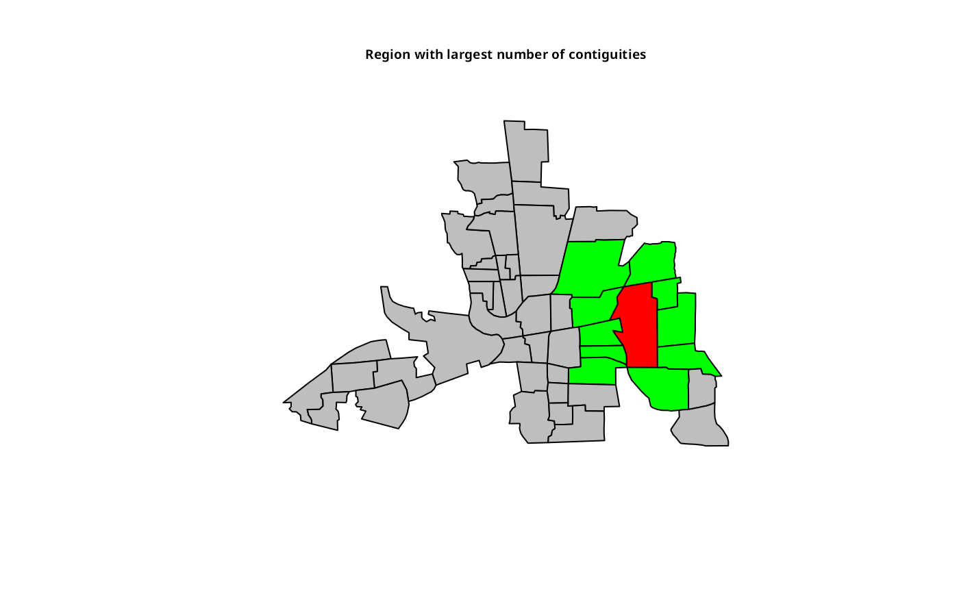
cards <- card(xx)
maxconts <- which(cards == max(cards))
if(length(maxconts) > 1) maxconts <- maxconts[1]
fg <- rep("grey", length(cards))
fg[maxconts] <- "red"
fg[xx[[maxconts]]] <- "green"
plot(st_geometry(columbus), col=fg)
title(main="Region with largest number of contiguities", cex.main=0.6)

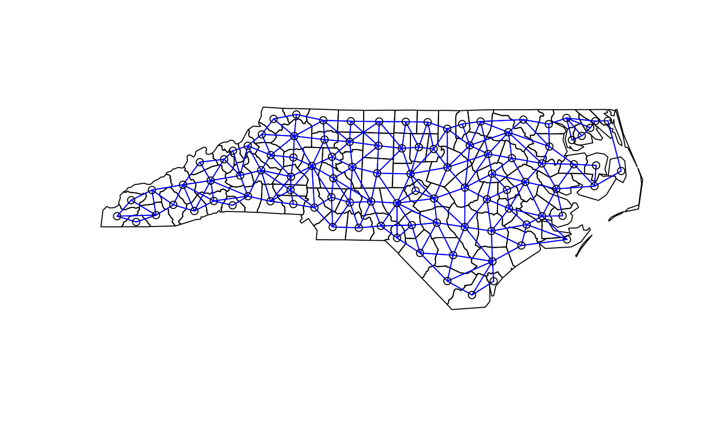
nc.sids <- st_read(system.file("shapes/sids.gpkg", package="spData")[1], quiet=TRUE)
system.time(xxnb <- poly2nb(nc.sids))
#>    user  system elapsed 
#>   0.041   0.000   0.041 
system.time(xxnb <- poly2nb(as(nc.sids, "Spatial")))
#>    user  system elapsed 
#>   0.055   0.000   0.055 
plot(st_geometry(nc.sids))
plot(xxnb, st_coordinates(st_centroid(nc.sids)), add=TRUE, col="blue")
#> Warning: st_centroid assumes attributes are constant over geometries

sq <- st_polygon(list(rbind(c(0,0), c(1,0), c(1,1), c(0,1), c(0,0))))
sq2 <- sq + c(0,1)
sq3 <- sq + c(1,0)
sq4 <- sq + c(1,1)
gm <- st_sfc(list(sq, sq2, sq3, sq4))
df <- st_as_sf(data.frame(gm, id=1:4))
plot(st_geometry(df))
text(st_coordinates(st_centroid(gm)), as.character(df$id))

unclass(poly2nb(df, queen = FALSE))
#> [[1]]
#> [1] 2 3
#> 
#> [[2]]
#> [1] 1 4
#> 
#> [[3]]
#> [1] 1 4
#> 
#> [[4]]
#> [1] 2 3
#> 
#> attr(,"region.id")
#> [1] "1" "2" "3" "4"
#> attr(,"call")
#> poly2nb(pl = df, queen = FALSE)
#> attr(,"type")
#> [1] "rook"
#> attr(,"snap")
#> [1] 1.490116e-08
#> attr(,"sym")
#> [1] TRUE
#> attr(,"ncomp")
#> attr(,"ncomp")$nc
#> [1] 1
#> 
#> attr(,"ncomp")$comp.id
#> [1] 1 1 1 1
#> 
col_geoms <- st_geometry(columbus)
col_geoms[1] <- st_buffer(col_geoms[1], dist=-0.05)
st_geometry(columbus) <- col_geoms
poly2nb(columbus)
#> Warning: some observations have no neighbours;
#> if this seems unexpected, try increasing the snap argument.
#> Warning: neighbour object has 2 sub-graphs;
#> if this sub-graph count seems unexpected, try increasing the snap argument.
#> Neighbour list object:
#> Number of regions: 49 
#> Number of nonzero links: 232 
#> Percentage nonzero weights: 9.662641 
#> Average number of links: 4.734694 
#> 1 region with no links:
#> 1
#> 2 disjoint connected subgraphs