Global Empirical Bayes estimator

The function computes global empirical Bayes estimates for rates "shrunk" to the overall mean.

EBest(n, x, family="poisson")

Arguments

n

a numeric vector of counts of cases

x

a numeric vector of populations at risk

family

either "poisson" for rare conditions or "binomial" for non-rare conditions

Details

Details of the implementation for the "poisson" family are to be found in Marshall, p. 284--5, and Bailey and Gatrell p. 303--306 and exercise 8.2, pp. 328--330. For the "binomial" family, see Martuzzi and Elliott (implementation by Olaf Berke).

Value

A data frame with two columns:

raw

a numerical vector of raw (crude) rates

estmm

a numerical vector of empirical Bayes estimates

and a parameters attribute list with components:

a

global method of moments phi value

m

global method of moments gamma value

References

Marshall R M (1991) Mapping disease and mortality rates using Empirical Bayes Estimators, Applied Statistics, 40, 283--294; Bailey T, Gatrell A (1995) Interactive Spatial Data Analysis, Harlow: Longman, pp. 303--306, Martuzzi M, Elliott P (1996) Empirical Bayes estimation of small area prevalence of non-rare conditions, Statistics in Medicine 15, 1867--1873.

Author

Roger Bivand Roger.Bivand@nhh.no and Olaf Berke, Population Medicine, OVC, University of Guelph, CANADA

See also

EBlocal, probmap, EBImoran.mc

Examples

auckland <- st_read(system.file("shapes/auckland.shp", package="spData")[1], quiet=TRUE)
res <- EBest(auckland$M77_85, 9*auckland$Und5_81)
attr(res, "parameters")
#> $a
#> [1] 7.284173e-07
#> 
#> $b
#> [1] 0.002633436
#> 
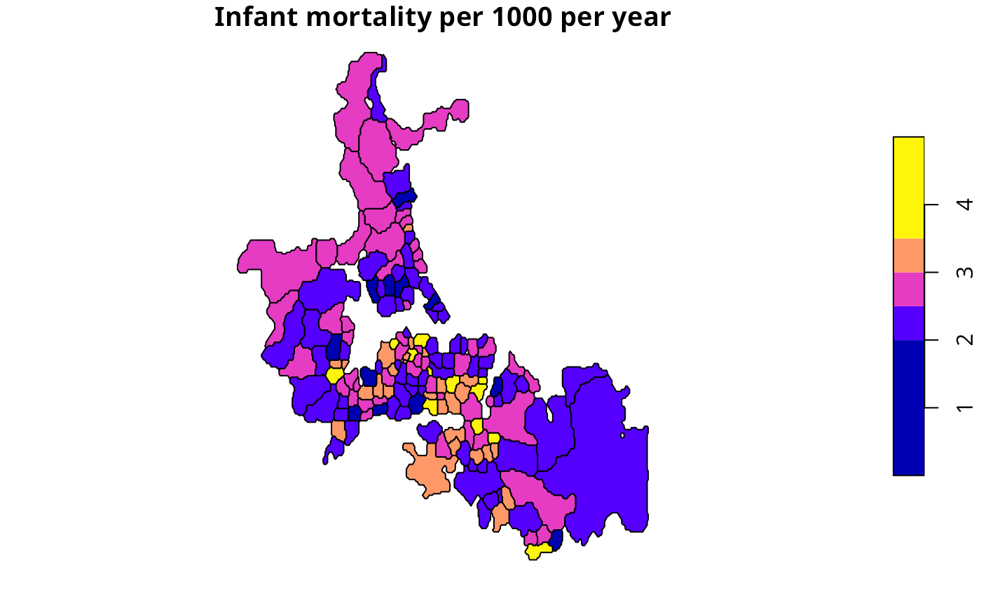
auckland$estmm000 <- res$estmm*1000
plot(auckland[,"estmm000"], breaks=c(0,2,2.5,3,3.5,5),
 main="Infant mortality per 1000 per year")

data(huddersfield, package="spData")
res <- EBest(huddersfield$cases, huddersfield$total, family="binomial")
round(res[,1:2],4)*100
#>      raw estmm
#> 1  42.86 34.44
#> 2  28.95 29.56
#> 3  28.31 28.94
#> 4  21.43 28.93
#> 5  33.33 30.72
#> 6  30.86 30.43
#> 7  33.70 31.85
#> 8  45.61 35.93
#> 9  26.67 28.95
#> 10 29.41 29.95
#> 11 27.76 28.36
#> 12 33.75 31.75
#> 13 32.67 31.84
#> 14 22.91 25.36
#> 15 34.21 32.33
#> 16 33.77 31.72
#> 17 29.09 29.69
#> 18 15.87 24.36
#> 19 40.91 32.11
#> 20 40.00 31.01
#> 21 28.79 29.53
#> 22 38.89 31.47
#> 23 28.32 29.10
#> 24 33.33 31.44
#> 25 13.95 22.36
#> 26 33.77 31.72
#> 27 31.58 30.31
#> 28 33.33 30.42
#> 29 26.67 28.26
#> 30 63.64 33.57
#> 31 34.38 32.24
#> 32 20.00 27.62
#> 33 19.15 24.60
#> 34 25.53 28.54
#> 35 24.14 27.79
#> 36 44.00 32.98
#> 37 25.33 27.95
#> 38 18.18 26.96
#> 39 31.78 30.97
#> 40 32.20 30.88
#> 41 26.19 28.23
#> 42 19.05 26.65
#> 43 16.67 26.81
#> 44 20.00 28.66
#> 45 32.99 31.54
#> 46 50.00 31.97
#> 47 37.21 32.30
#> 48 32.79 31.13
#> 49 38.89 31.47
#> 50 25.00 27.26
#> 51 26.03 28.29
#> 52 30.43 30.18
#> 53 19.75 25.28
#> 54 50.00 31.61
#> 55 21.62 27.67
#> 56 22.22 27.88
#> 57 36.36 30.71
#> 58 31.25 30.22
#> 59  0.00 29.73
#> 60 29.41 29.95
#> 61 31.16 30.71
#> 62 33.33 30.58
#> 63 33.87 32.22
#> 64 30.00 30.04
#> 65 30.34 30.19
#> 66 40.74 35.00
#> 67 46.43 38.96
#> 68 34.21 31.91
#> 69 24.26 26.10
#> 70 29.41 29.75
#> 71 47.17 39.13