No-neighbour observation and subgraph handling

Introduction

The spdep package has always been careful about disconnected graphs, especially where the disconnected observations are graph nodes with no neighbours, that is no incoming or outgoing edges. In nb neighbour objects, they are encoded as integer vectors of length 1 containing integer 0, which is an invalid index on $[1, N]$ , where $N$ is the observation count. Functions taking neighbour objects as arguments use the zero.policy argument to guide how to handle no-neighbour observations.

spdep has also had n.comp.nb to find the number of disjoint connected subgraphs in an nb object, contributed by Nicholas Lewin-Koh in 2001 and using depth-first search for symmetric neighbours, showing in addition which observations belong to which subgraph. Obviously, no-neighbour observations are singleton graph nodes, but subgraphs are also troubling for spatial analysis, because there is no connection between the spatial processes in those subgraphs. The ripples in one pond cannot cross into a separate pond if they are not connected.

From spdep 1.3-1, steps began to raise awareness of the possibility that neighbour objects might be created that are disconnected in some way, mostly through warnings, and through the computation of subgraph measures by default. This vignette is intended to provide some background to these steps.

No-neighbour observations

From the start, nb objects have recorded no-neighbour observations as an integer vector of unit length and value 0, where neighbours are recorded as ID values between 1 and N, where N is the observation count. print and summary methods have always reported the presence of no-neighbour observations, and listed their IDs (or region.id values). If an nb object contains no-neighbour observations, the user has to decide whether to drop those observations, or if retained, what value to give its weights. The zero.policy argument uses zero as the value if TRUE, but if FALSE causes nb2listw to fail. The value of zero.policy in a call to functions like nb2listw, subset.listw or mat2listw creating listw objects representing sparse spatial weights matrices is added to the created object as an attribute, and used subsequently to pass through that choice to other functions. For example, moran.test takes the value of this attribute as default for its zero.policy argument:

library(spdep)

## Loading required package: spData

## Loading required package: sf

## Linking to GEOS 3.13.0, GDAL 3.9.2, PROJ 9.5.0; sf_use_s2() is TRUE

args(moran.test)

## function (x, listw, randomisation = TRUE, zero.policy = attr(listw, 
##     "zero.policy"), alternative = "greater", rank = FALSE, na.action = na.fail, 
##     spChk = NULL, adjust.n = TRUE, drop.EI2 = FALSE) 
## NULL

If observation $i$ has no neighbours, its weights sum $\sum_{j=1}^N w_{ij} = 0$ , as $w_{ij} = 0, \forall j$ (see discussion in Bivand and Portnov (2004)). Its eigenvalue will also be zero, with consequences for analytical inference:

eigen(0)$values

## [1] 0

The adjust.n argument to measures of spatial autocorrelation is by default TRUE, and subtracts the count of singleton nodes from $N$ in an attempt to acknowledge the reduction in information available.

This discussion will address problems arising when analysing areal/lattice data, and neighbours are defined as polygon features with contiguous boundaries. One way in which no-neighbour observations may occur is when they are islands. This is clearly the case in Freni-Sterrantino, Ventrucci, and Rue (2018), where Capraia and Giglio Isles are singleton nodes. Here we take Westminster constituencies for Wales used in the July 2024 UK general election. If GDAL is at least version 3.7.0, the driver supports compressed GeoPackage files, if not they must be decompressed first.

(GDAL37 <- as.numeric_version(unname(sf_extSoftVersion()["GDAL"])) >= "3.7.0")

## [1] TRUE

The boundaries are taken from the Ordnance Survey Boundary-Line site, https://osdatahub.os.uk/downloads/open/BoundaryLine, choosing the 2024 Westminster constituencies (https://www.os.uk/opendata/licence), simplified using a tolerance of 50m to reduce object size, and merged with selected voting outcomes for constituencies in Great Britain https://electionresults.parliament.uk/countries/1, (https://www.nationalarchives.gov.uk/doc/open-government-licence/version/3/). Here, the subset for Wales is useful as we will see:

file <- "etc/shapes/GB_2024_Wales_50m.gpkg.zip"
zipfile <- system.file(file, package="spdep")
if (GDAL37) {
    w50m <- st_read(zipfile)
} else {
    td <- tempdir()
    bn <- sub(".zip", "", basename(file), fixed=TRUE)
    target <- unzip(zipfile, files=bn, exdir=td)
    w50m <- st_read(target)
}

## Reading layer `GB_2024_Wales_50m' from data source 
##   `/tmp/RtmpqhccSk/temp_libpath108a2257736002/spdep/etc/shapes/GB_2024_Wales_50m.gpkg.zip' 
##   using driver `GPKG'
## Simple feature collection with 32 features and 19 fields
## Geometry type: MULTIPOLYGON
## Dimension:     XY
## Bounding box:  xmin: 146597.1 ymin: 164536.5 xmax: 355287 ymax: 395993.5
## Projected CRS: OSGB36 / British National Grid

(w50m |> poly2nb(row.names=as.character(w50m$Constituency)) -> nb_W_50m)

## Warning in poly2nb(w50m, row.names = as.character(w50m$Constituency)): some observations have no neighbours;
## if this seems unexpected, try increasing the snap argument.

## Warning in poly2nb(w50m, row.names = as.character(w50m$Constituency)): neighbour object has 2 sub-graphs;
## if this sub-graph count seems unexpected, try increasing the snap argument.

## Neighbour list object:
## Number of regions: 32 
## Number of nonzero links: 136 
## Percentage nonzero weights: 13.28125 
## Average number of links: 4.25 
## 1 region with no links:
## Ynys Môn
## 2 disjoint connected subgraphs

The two subgraphs are the singleton Ynys Môn and all the other 31 constituencies:

attr(nb_W_50m, "ncomp")$comp.id |>table() |> table()

## 
##  1 31 
##  1  1

The left map shows that Ynys Môn can be shown selecting by name, as a black border, and by the zero cardinality of its neighbour set, using card, filling the polygon. The right map shows the location of the island, known in English as Anglesey, north-west of the Welsh mainland, and with no neighbour links:

ynys_mon <- w50m$Constituency == "Ynys Môn"
pts <- st_point_on_surface(st_geometry(w50m))
opar <- par(mfrow=c(1, 2))
plot(st_geometry(w50m), border="grey75")
plot(st_geometry(w50m)[ynys_mon], add=TRUE)
plot(st_geometry(w50m)[card(nb_W_50m) == 0L], add=TRUE, border="transparent", col="wheat1")
plot(st_geometry(w50m), border="grey75")
plot(nb_W_50m, pts, add=TRUE)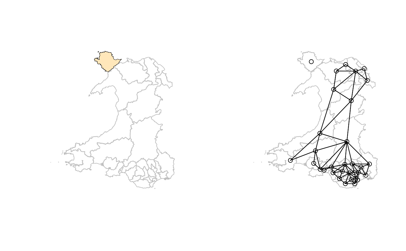

par(opar)

From the maps, we can see that the island is close to two constituencies across the Afon Menai (Menai Strait in English), the three simplified polygons being less than 280m apart, measured between polygon boundaries:

dym <- c(st_distance(w50m[ynys_mon,], w50m))
sort(dym)[1:12]

## Units: [m]
##  [1]      0.0000    123.4132    277.5414  16658.7265  37985.7086  54096.7729
##  [7]  58146.4320  65550.2491  67696.3323  93741.9873 113007.3659 137858.1826

Using a snap distance of 280m, we can join the island to its two obvious proximate neighbours:

(nb_W_50m_snap <- poly2nb(w50m, row.names=as.character(w50m$Constituency), snap=280))

## Neighbour list object:
## Number of regions: 32 
## Number of nonzero links: 140 
## Percentage nonzero weights: 13.67188 
## Average number of links: 4.375

plot(st_geometry(w50m), border="grey75")
plot(nb_W_50m_snap, pts, add=TRUE)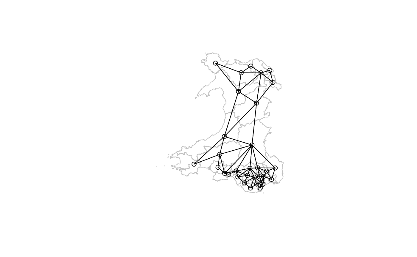

In this case, increasing snap from its default of 10mm (or close equivalents for geometries with known metrics; previously sqrt(.Machine$double.eps) 1.4901161^{-8} in all cases) helps. The symmetric links added are to:

attr(nb_W_50m_snap, "region.id")[nb_W_50m_snap[[which(ynys_mon)]]]

## [1] "Bangor Aberconwy"   "Dwyfor Meirionnydd"

This is not always going to be the case, but here the strait is narrow. If islands are much further offshore, other steps may be required, because a large snap distance will draw in extra neighbours for already connected observations. It is also possible that increasing the snap distance may fail to link islands if they are not considered candidate neighbours, that is if their extents (bounding boxes), buffered out by the snap value, do not intersect.

We can also use the distances to pick out those neighbour candidates that meet our criterion of 280m, taking care not to lose the ordering needed to identify the correct observations:

(meet_criterion <- sum(dym <= units::set_units(280, "m")))

## [1] 3

These candidates are the island itself, and the two neighbours across the Menai Strait:

(cands <- attr(nb_W_50m, "region.id")[order(dym)[1:meet_criterion]])

## [1] "Ynys Môn"           "Bangor Aberconwy"   "Dwyfor Meirionnydd"

The addlinks1 function can be used to add both the links from Ynys Môn to its neighbours, and by symmetry from them to Ynys Môn. This approach means that each island should be treated separately (or scripted in sequence), but does not risk adding spurious neighbours in denser parts of the study area.

(nb_W_50m_add <- addlinks1(nb_W_50m, from = cands[1], to = cands[2:meet_criterion]))

## Neighbour list object:
## Number of regions: 32 
## Number of nonzero links: 140 
## Percentage nonzero weights: 13.67188 
## Average number of links: 4.375

all.equal(nb_W_50m_add, nb_W_50m_snap, check.attributes=FALSE)

## [1] TRUE

Since these constituency observations have areal support, it is not surprising that changing support to points and using $k$ -nearest neighbours does not work adequately, because the distance measurements are between the points representing the polygons rather than as above between the areal unit boundaries:

k2 <- knn2nb(knearneigh(pts, k=2), row.names=as.character(w50m$Constituency), sym=TRUE)

## Warning in knn2nb(knearneigh(pts, k = 2), row.names =
## as.character(w50m$Constituency), : neighbour object has 2 sub-graphs

attr(k2, "region.id")[k2[[which(ynys_mon)]]]

## [1] "Bangor Aberconwy" "Clwyd North"

Here, Clwyd North, east of Bangor Aberconwy, is given as a neighbour of Ynys Môn but Dwyfor Meirionnydd, west of Bangor Aberconwy, is not. In addition, there are two subgraphs, which still remain up to $k=6$ .

Subgraphs

Subgraphs may be found when no-neighbour observations are present, but also when the graph is split between two blocks of observations with no path from any observation in a block to any in another block, across the low population density constituencies in mid-Wales:

(k6 <- knn2nb(knearneigh(pts, k=6), row.names=as.character(w50m$Constituency), sym=TRUE))

## Warning in knn2nb(knearneigh(pts, k = 6), row.names =
## as.character(w50m$Constituency), : neighbour object has 2 sub-graphs

## Neighbour list object:
## Number of regions: 32 
## Number of nonzero links: 238 
## Percentage nonzero weights: 23.24219 
## Average number of links: 7.4375 
## 2 disjoint connected subgraphs

plot(st_geometry(w50m), border="grey75")
plot(k6, pts, add=TRUE)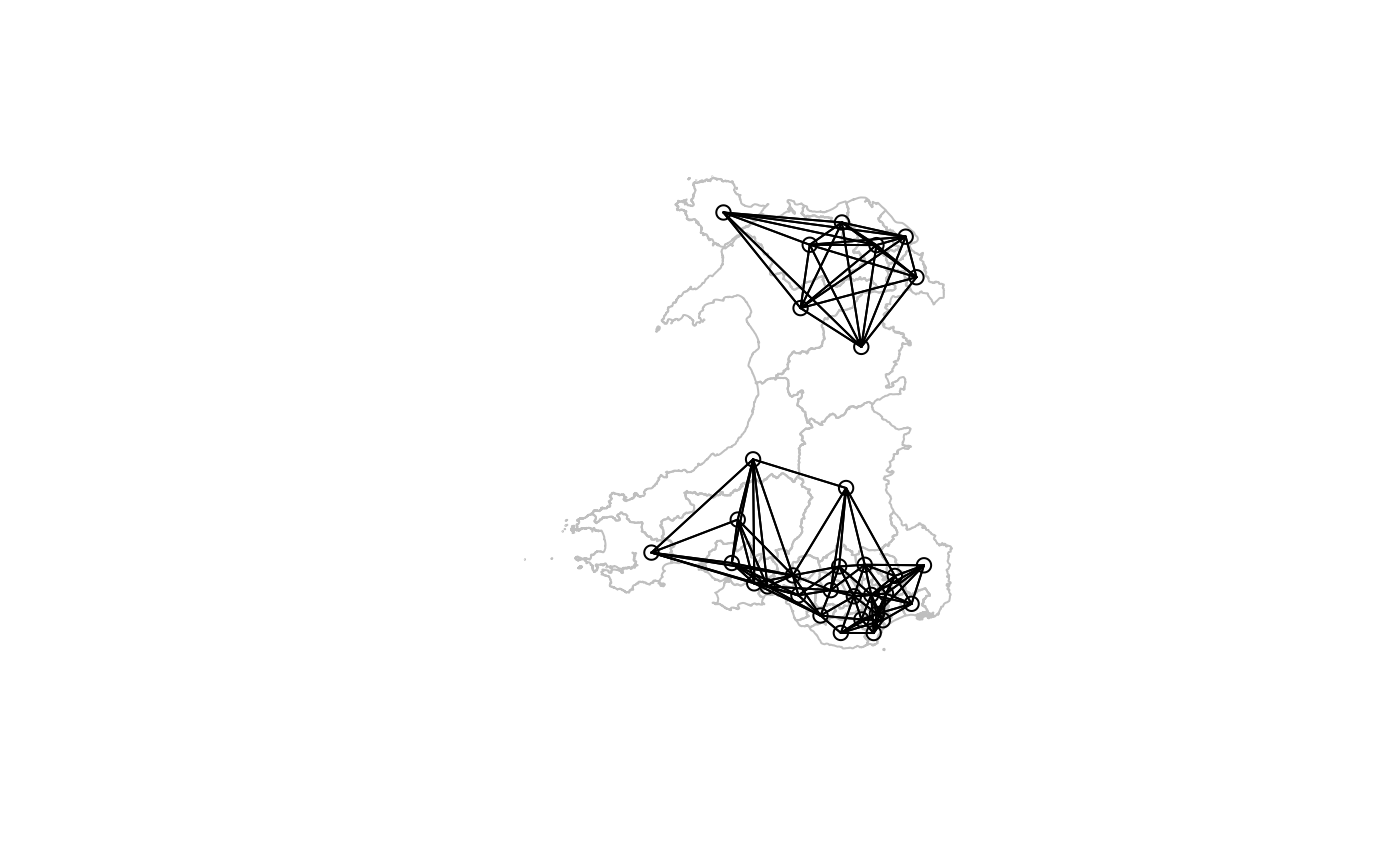

We can show the block structure by displaying the binary spatial weights matrix:

o <- order(attr(k6, "ncomp")$comp.id)
image(t(nb2mat(k6, style="B")[o, rev(o)]), axes=FALSE, asp=1)

This occurs frequently with point support, but may also occur with areal support, as Freni-Sterrantino, Ventrucci, and Rue (2018) find for the eight municipalities on the island of Elba.

From spdep 1.3-6, if the igraph and spatialreg packages are available, n.comp.nb uses igraph::components to compute the graph components, also using depth-first search. The original implementation is as fast, but for directed (asymmetric) graphs converts first to symmetry, while igraph::components can handle directed graphs without such conversion (see https://github.com/r-spatial/spdep/issues/160 for details).

(k6a <- knn2nb(knearneigh(pts, k=6), row.names=as.character(w50m$Constituency)))

## Warning in knn2nb(knearneigh(pts, k = 6), row.names =
## as.character(w50m$Constituency)): neighbour object has 2 sub-graphs

## Neighbour list object:
## Number of regions: 32 
## Number of nonzero links: 192 
## Percentage nonzero weights: 18.75 
## Average number of links: 6 
## 2 disjoint connected subgraphs
## Non-symmetric neighbours list

Another case demonstrates how cyclical subgraphs may appear; this is again taken from constituencies in the 2024 UK general election, subsetted to those in England south of London.

file <- "etc/shapes/GB_2024_southcoast_50m.gpkg.zip"
zipfile <- system.file(file, package="spdep")
if (GDAL37) {
    sc50m <- st_read(zipfile)
} else {
    td <- tempdir()
    bn <- sub(".zip", "", basename(file), fixed=TRUE)
    target <- unzip(zipfile, files=bn, exdir=td)
    sc50m <- st_read(target)
}

## Reading layer `GB_2024_southcoast_50m' from data source 
##   `/tmp/RtmpqhccSk/temp_libpath108a2257736002/spdep/etc/shapes/GB_2024_southcoast_50m.gpkg.zip' 
##   using driver `GPKG'
## Simple feature collection with 119 features and 19 fields
## Geometry type: MULTIPOLYGON
## Dimension:     XY
## Bounding box:  xmin: 82643.12 ymin: 5342.9 xmax: 640301.6 ymax: 187226.2
## Projected CRS: OSGB36 / British National Grid

(nb_sc_50m <- poly2nb(sc50m, row.names=as.character(sc50m$Constituency)))

## Warning in poly2nb(sc50m, row.names = as.character(sc50m$Constituency)): neighbour object has 2 sub-graphs;
## if this sub-graph count seems unexpected, try increasing the snap argument.

## Neighbour list object:
## Number of regions: 119 
## Number of nonzero links: 530 
## Percentage nonzero weights: 3.742674 
## Average number of links: 4.453782 
## 2 disjoint connected subgraphs

The second subgraph only has two members, who are each others’ only neighbours, known as a cyclical component.

nc <- attr(nb_sc_50m, "ncomp")$comp.id
table(nc)

## nc
##   1   2 
## 117   2

Both constituencies are on the Isle of Wight:

(sub2 <- attr(nb_sc_50m, "region.id")[nc == 2L])

## [1] "Isle of Wight East" "Isle of Wight West"

pts <- st_point_on_surface(st_geometry(sc50m))
plot(st_geometry(sc50m), border="grey75")
plot(st_geometry(sc50m)[nc == 2L], border="orange", lwd=2, add=TRUE)
plot(nb_sc_50m, pts, add=TRUE)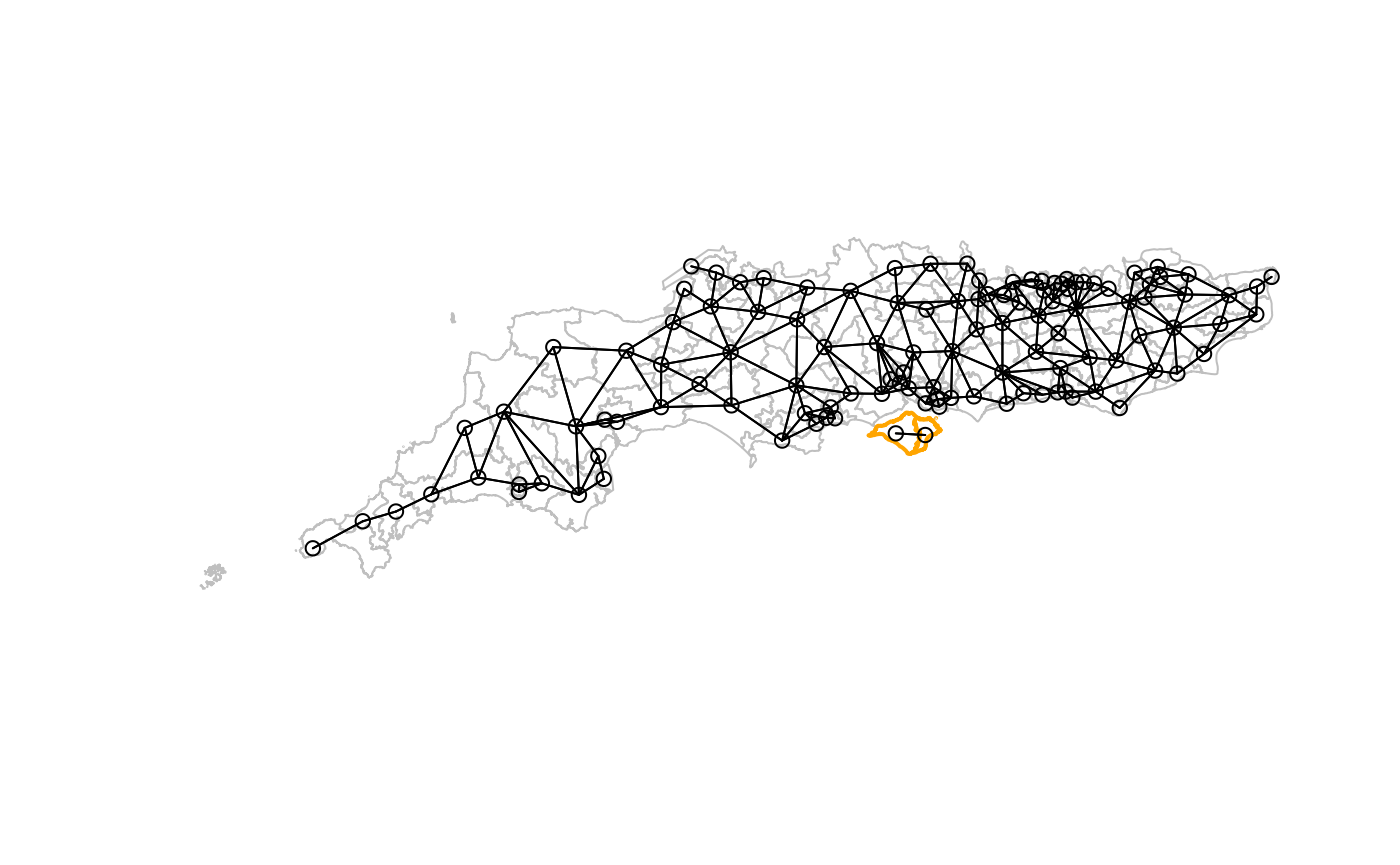

This has consequences for the eigenvalues of the spatial weights matrix, pointed out by Smirnov and Anselin (2009) and Bivand, Hauke, and Kossowski (2013). With row-standardised weights, the eigenvalues of this component are:

1/range(eigen(cbind(c(0, 1), c(1, 0)))$values)

## [1] -1  1

1/range(eigen(nb2mat(subset(nb_sc_50m, nc == 2L), style="W"))$values)

## [1] -1  1

This “takes over” the lower domain boundary, which for the whole data set is now the same:

1/range(eigen(nb2mat(nb_sc_50m, style="W"))$values)

## [1] -1  1

compared to the lower domain boundary for the remainder of the study area:

1/range(eigen(nb2mat(subset(nb_sc_50m, nc == 1L), style="W"))$values)

## [1] -1.094637  1.000000

This subgraph may be added to the remainder as shown above:

iowe <- match(sub2[1], attr(nb_sc_50m, "region.id"))
diowe <- c(st_distance(sc50m[iowe,], sc50m))
sort(diowe)[1:12]

## Units: [m]
##  [1]     0.000     0.000  1886.833  3509.366  6693.575  6943.672  7678.999
##  [8]  8576.454 10579.530 12163.332 16875.920 17161.786

ioww <- match(sub2[2], attr(nb_sc_50m, "region.id"))
dioww <- c(st_distance(sc50m[ioww,], sc50m))
sort(dioww)[1:12]

## Units: [m]
##  [1]     0.000     0.000  1232.724  2541.318  5746.764  5770.602  8902.579
##  [8]  9747.265 10529.540 10909.845 12250.564 12379.871

Using 5km as a cutoff seems prudent, but would not work as a snap value. Taking Isle of Wight East first, there are four constituencies with boundaries within 5km:

(meet_criterion <- sum(diowe <= units::set_units(5000, "m")))

## [1] 4

Obviously the contiguous neighbour is among them with zero distance, and needs to be dropped, although addlinks1 would drop the duplicate:

(cands <- attr(nb_sc_50m, "region.id")[order(diowe)[1:meet_criterion]])

## [1] "Isle of Wight East" "Isle of Wight West" "Portsmouth South"  
## [4] "Gosport"

(nb_sc_50m_iowe <- addlinks1(nb_sc_50m, from = cands[1], to = cands[3:meet_criterion]))

## Neighbour list object:
## Number of regions: 119 
## Number of nonzero links: 534 
## Percentage nonzero weights: 3.77092 
## Average number of links: 4.487395

Although all constituencies are now linked, we should see whether using the 5km criterion brings in extra neighbours for Isle of Wight West:

(meet_criterion <- sum(dioww <= units::set_units(5000, "m")))

## [1] 4

It, does, but we need to beware of the sorting order of the zero self-distance and contiguous neighbour distance, where from is now in the second position:

(cands <- attr(nb_sc_50m, "region.id")[order(dioww)[1:meet_criterion]])

## [1] "Isle of Wight East" "Isle of Wight West" "New Forest West"   
## [4] "New Forest East"

This then yields links to the north-west:

(nb_sc_50m_iow <- addlinks1(nb_sc_50m_iowe, from = cands[2], to = cands[3:meet_criterion]))

## Neighbour list object:
## Number of regions: 119 
## Number of nonzero links: 538 
## Percentage nonzero weights: 3.799167 
## Average number of links: 4.521008

pts <- st_point_on_surface(st_geometry(sc50m))
plot(st_geometry(sc50m), border="grey75")
plot(st_geometry(sc50m)[nc == 2L], border="orange", lwd=2, add=TRUE)
plot(nb_sc_50m_iow, pts, add=TRUE)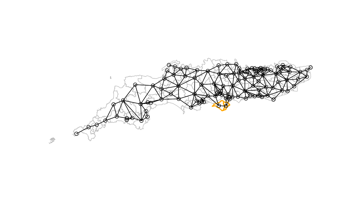

It remains to add a suitable generalisation of addlinks1 to handle a from vector argument and a to argument taking a list of vectors.

Per-session control of function behaviour

From very early on, the default value of the zero.policy argument to many methods and functions was NULL. If the value was NULL, zero.policy would be set from get.ZeroPolicyOption:

get.ZeroPolicyOption()

## [1] FALSE

On loading spdep, the internal option is set to FALSE, so functions and methods using zero.policy need to choose how to handle islands:

try(nb2listw(nb_W_50m))

## Error in nb2listw(nb_W_50m) : 
##   Empty neighbour sets found (zero.policy: FALSE)

In this case, it was shown above how the island may reasonably be associated with proximate constituencies on the mainland. If, however, the user wishes to override the default, set.ZeroPolicyOption may be used to set a different per-session default:

set.ZeroPolicyOption(TRUE)

get.ZeroPolicyOption()

## [1] TRUE

(lw <- nb2listw(nb_W_50m))

## Characteristics of weights list object:
## Neighbour list object:
## Number of regions: 32 
## Number of nonzero links: 136 
## Percentage nonzero weights: 13.28125 
## Average number of links: 4.25 
## 1 region with no links:
## Ynys Môn
## 2 disjoint connected subgraphs
## 
## Weights style: W 
## Weights constants summary:
##    n  nn S0       S1      S2
## W 31 961 31 15.36355 129.051

attr(lw, "zero.policy")

## [1] TRUE

set.ZeroPolicyOption(FALSE)

When a listw object is created with zero.policy set to TRUE, this choice is added to the output object as an attribute and applied when the object is used (unless specifically overridden). Note also above that while there are 32 constituencies, the observation count reported by spweights.constants called by the print method for listw object has argument adjust.n TRUE, dropping no-neighbour observations from the observation count.

Other internal options have been introduced to suppress no-neighbour and subgraph warnings when creating nb objects. The default values are as follows:

get.NoNeighbourOption()

## [1] TRUE

get.SubgraphOption()

## [1] TRUE

get.SubgraphCeiling()

## [1] 100000

get.NoNeighbourOption controls the issuing of warnings when nb objects are created with no-neighbour observations; get.SubgraphOption works similarly but for warnings issued when there is more than one graph component; both are TRUE by default. get.SubgraphCeiling sets the integer value of graph nodes plus graph edges above which calculating on the graph is considered too costly in compute time, the default is 100,000. This corresponds to a dense neighbour set with just over 300 nodes (with almost 100000 edges) such as that needed to use inverse distance weights, or just over 14,000 nodes with an average neighbour count of 6.

The print method for nb objects reports no-neighbour and subgraph status anyway, so careful users who always examine generated objects may prefer to supress the warnings, but warnings seem prudent when users may not examine the objects, or when generation is by subsetting of larger objects, for example in the creation of training and test data sets. Here the Welsh constituency boundaries will be used to show the behaviour of the internal options:

set.NoNeighbourOption(FALSE)
(w50m |> poly2nb(row.names=as.character(w50m$Constituency)) -> nb_W_50mz)

## Warning in poly2nb(w50m, row.names = as.character(w50m$Constituency)): neighbour object has 2 sub-graphs;
## if this sub-graph count seems unexpected, try increasing the snap argument.

## Neighbour list object:
## Number of regions: 32 
## Number of nonzero links: 136 
## Percentage nonzero weights: 13.28125 
## Average number of links: 4.25 
## 1 region with no links:
## Ynys Môn
## 2 disjoint connected subgraphs

Turning both off removes the warnings:

set.SubgraphOption(FALSE)
(w50m |> poly2nb(row.names=as.character(w50m$Constituency)) -> nb_W_50my)

## Neighbour list object:
## Number of regions: 32 
## Number of nonzero links: 136 
## Percentage nonzero weights: 13.28125 
## Average number of links: 4.25 
## 1 region with no links:
## Ynys Môn

When get.SubgraphOption is FALSE, the attribute containing the output of n.comp.nb is not added:

str(attr(nb_W_50my, "ncomp"))

##  NULL

The reduction of the ceiling to below node count 32 plus edge count 136 also supresses the calculation of graph components:

set.SubgraphOption(TRUE)
set.SubgraphCeiling(100L)
(w50m |> poly2nb(row.names=as.character(w50m$Constituency)) -> nb_W_50mx)

## Neighbour list object:
## Number of regions: 32 
## Number of nonzero links: 136 
## Percentage nonzero weights: 13.28125 
## Average number of links: 4.25 
## 1 region with no links:
## Ynys Môn

str(attr(nb_W_50mx, "ncomp"))

##  NULL

Restoring the remaining default values:

set.SubgraphCeiling(100000L)
set.NoNeighbourOption(TRUE)

Unintentional disconnected graphs

Sometimes apparently sensible polygons turn out to be represented in such a way that disconnected graphs are generated when extracting contiguities. One such case was raised in https://github.com/r-spatial/spdep/issues/162, for subdivisions of Tokyo. The original data file tokyomet262.* from https://sgsup.asu.edu/sites/default/files/SparcFiles/tokyo_0.zip was created some twenty years ago by Tomoki Nakaya and Martin Charlton, and some geometry issues were known at the time. A possibility that may affect legacy files is projection of geometries on 32-bit platforms, but it is not known whether this affected this file. Here it has been re-packaged as a compressed GeoPackage:

file <- "etc/shapes/tokyo.gpkg.zip"
zipfile <- system.file(file, package="spdep")
if (GDAL37) {
    tokyo <- st_read(zipfile)
} else {
    td <- tempdir()
    bn <- sub(".zip", "", basename(file), fixed=TRUE)
    target <- unzip(zipfile, files=bn, exdir=td)
    tokyo <- st_read(target)
}

## Reading layer `tokyo' from data source 
##   `/tmp/RtmpqhccSk/temp_libpath108a2257736002/spdep/etc/shapes/tokyo.gpkg.zip' 
##   using driver `GPKG'
## Simple feature collection with 262 features and 3 fields
## Geometry type: MULTIPOLYGON
## Dimension:     XY
## Bounding box:  xmin: 266206.6 ymin: -90932.11 xmax: 411400.3 ymax: 37142.75
## Projected CRS: Tokyo / Japan Plane Rectangular CS VI

After correcting invalid polygons:

all(st_is_valid(tokyo))

## [1] TRUE

tokyo <- st_make_valid(tokyo)

applying poly2nb with the legacy default snap value produced numerous singleton observations as well as many multiple-observation subgraphs:

(nb_t0 <- poly2nb(tokyo, snap=sqrt(.Machine$double.eps)))

## Warning in poly2nb(tokyo, snap = sqrt(.Machine$double.eps)): some observations have no neighbours;
## if this seems unexpected, try increasing the snap argument.

## Warning in poly2nb(tokyo, snap = sqrt(.Machine$double.eps)): neighbour object has 23 sub-graphs;
## if this sub-graph count seems unexpected, try increasing the snap argument.

## Neighbour list object:
## Number of regions: 262 
## Number of nonzero links: 946 
## Percentage nonzero weights: 1.378125 
## Average number of links: 3.610687 
## 10 regions with no links:
## 101, 127, 134, 135, 152, 154, 167, 237, 242, 243
## 23 disjoint connected subgraphs

The legacy default snap value when the coordinates are measured in metres was 15 nanometres, which effectively assumed that the coordinates making up polygon boundaries were identical:

units::set_units(units::set_units(attr(nb_t0, "snap"), "m"), "nm")

## 14.90116 [nm]

Stepping out a little to 2mm, the lack of contact ceased to be a problem.

(nb_t1 <- poly2nb(tokyo, snap=0.002))

## Neighbour list object:
## Number of regions: 262 
## Number of nonzero links: 1390 
## Percentage nonzero weights: 2.02494 
## Average number of links: 5.305344

units::set_units(units::set_units(attr(nb_t1, "snap"), "m"), "mm")

## 2 [mm]

On that basis, the default was changed from spdep 1.3-6 to 10mm for projected polygons, and the snap value used was returned as an attribute of the neighbour object:

(nb_t2 <- poly2nb(tokyo))

## Neighbour list object:
## Number of regions: 262 
## Number of nonzero links: 1390 
## Percentage nonzero weights: 2.02494 
## Average number of links: 5.305344

units::set_units(units::set_units(attr(nb_t2, "snap"), "m"), "mm")

## 10 [mm]

Where the polygons are represented by geographical (spherical) coordinates, the new default from spdep 1.3-6 is set to a value mimicking 10mm:

(nb_t3 <- poly2nb(st_transform(tokyo, "OGC:CRS84")))

## Neighbour list object:
## Number of regions: 262 
## Number of nonzero links: 1336 
## Percentage nonzero weights: 1.946274 
## Average number of links: 5.099237

The default snap value used in poly2nb when the polygons are expressed in decimal degrees is:

attr(nb_t3, "snap")

## [1] 9e-08

This was set based on the apparent “size” of 10mm in decimal degrees:

(180 * 0.01) / (pi * 6378137)

## [1] 8.983153e-08

References

Bivand, Roger, Jan Hauke, and Tomasz Kossowski. 2013. “Computing the Jacobian in Gaussian Spatial Autoregressive Models: An Illustrated Comparison of Available Methods.” Geographical Analysis 45 (2): 150–79. https://doi.org/10.1111/gean.12008.

Bivand, Roger, and B. A. Portnov. 2004. “Exploring Spatial Data Analysis Techniques Using R: The Case of Observations with No Neighbours.” In Advances in Spatial Econometrics: Methodology, Tools, Applications, edited by Luc Anselin, Raymond J. G. M. Florax, and S. J. Rey, 121–42. Berlin: Springer. https://doi.org/10.1007/978-3-662-05617-2_6.

Freni-Sterrantino, Anna, Massimo Ventrucci, and Håvard Rue. 2018. “A Note on Intrinsic Conditional Autoregressive Models for Disconnected Graphs.” Spatial and Spatio-Temporal Epidemiology 26: 25–34. https://doi.org/10.1016/j.sste.2018.04.002.

Smirnov, O., and L. Anselin. 2009. “An O(N) Parallel Method of Computing the Log-Jacobian of the Variable Transformation for Models with Spatial Interaction on a Lattice.” Computational Statistics & Data Analysis 53 (8): 2980–88. https://doi.org/10.1016/j.csda.2008.10.010.