1. The problem
GEE offers on-the-fly computation for rendering EE spatial objects:
library(rgee)
library(rgeeExtra)

ee_Initialize()

img <- ee$Image$Dataset$CGIAR_SRTM90_V4
Map$addLayer(log1p(img), list(min = 0, max = 7))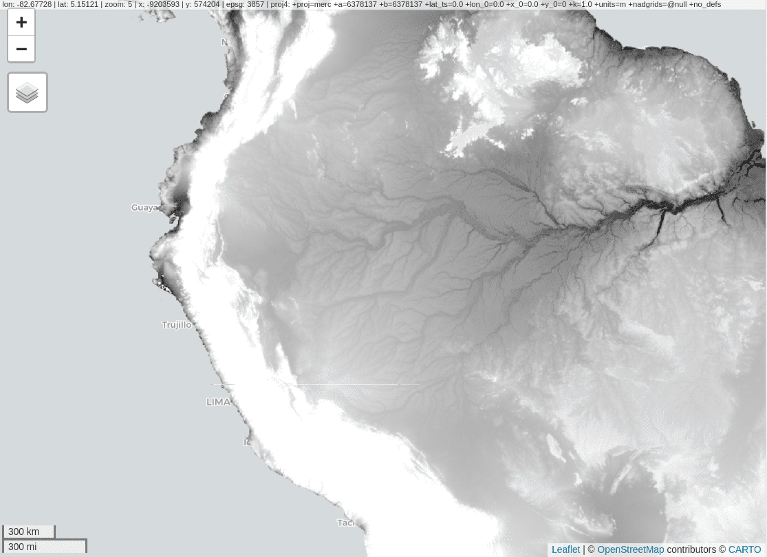
However, this interactive map service is temporary,
disappearing after a short period of time (~ 4 hours). This makes
Map$addLayer unusable for report generation. In this
vignette, we will learn to create a permanent interactive
map.
2. A tentative workaround
Instead of using GEE API for creating interactive maps, we will use titiler. titiler creates web map tiles dynamically based on COG (STAC) resources. Since an exported EE task to retrieve images can return a COG, we just have to move these results to a storage web service with HTTP GET range requests.
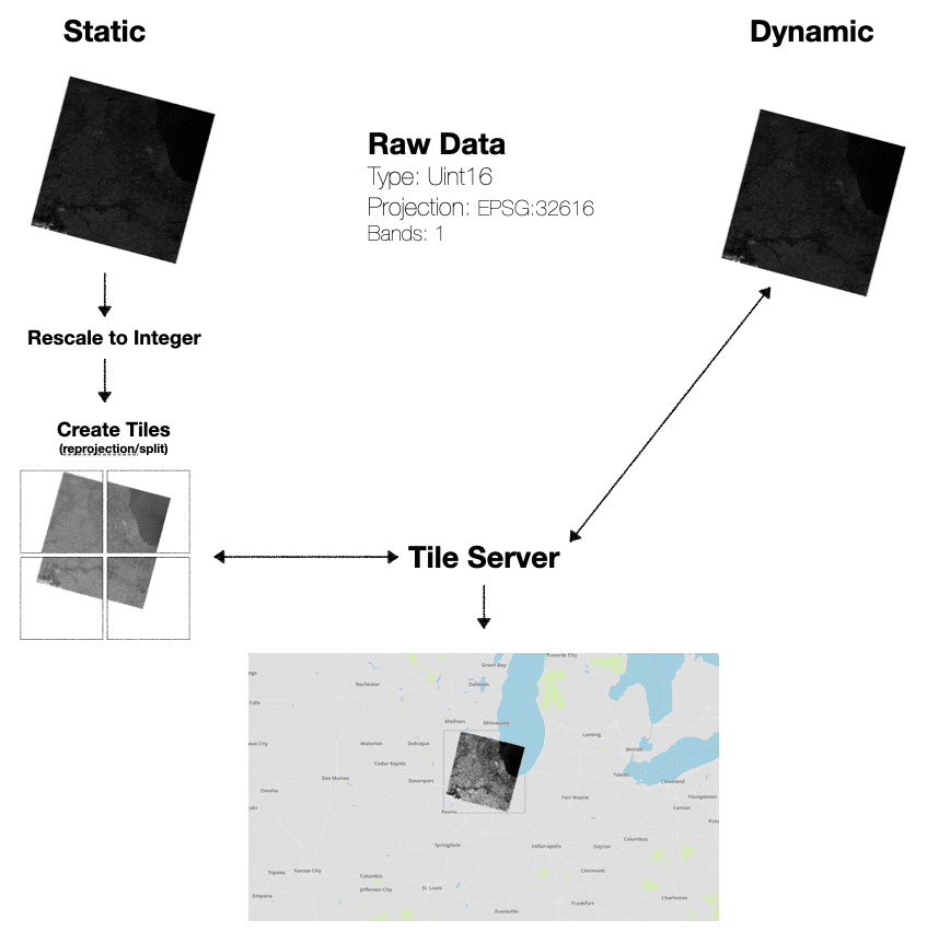
Fortunately, GCS counts with this feature, so if we manage to move our results to GCS, the work would be already done :)
GET /OBJECT_NAME HTTP/1.1
Host: BUCKET_NAME.storage.googleapis.com
Content-Length: 0
Authorization: AUTHENTICATION_STRING
Range: bytes=BYTE_RANGE
If-Match: ENTITY_TAG
If-Modified-Since: DATE
If-None-Match: ENTITY_TAG
If-Unmodified-Since: DATE
3. Show me the code!
First, load rgee and googleCloudStorageR
and initialize the EE API. You must have correctly configured a service
account key, if not check our tutorial “how
to integrate Google Cloud Storage and rgee”.
library(rgee)
library(googleCloudStorageR)

# Init the EE API
ee_Initialize("csaybar", gcs = TRUE)

# Validate your SaK
# ee_utils_sak_validate(bucket = "rgee_examples")
Define your study area.
# Define an study area
EE_geom <- ee$Geometry$Point(c(-70.06240, -6.52077))$buffer(5000)
Select an ee$Image, for instance, a Landsat-8 image.
l8img <- ee$ImageCollection$Dataset$LANDSAT_LC08_C02_T2_L2 %>%
  ee$ImageCollection$filterDate('2021-06-01', '2021-12-01') %>%
  ee$ImageCollection$filterBounds(EE_geom) %>%
  ee$ImageCollection$first()
Move l8img from EE to GCS.
gcs_l8_name  <- "l8demo2" # name of the image in GCS.
BUCKET_NAME <- "rgee_examples" # set here your bucket name
task <- ee_image_to_gcs(
  image = l8img$select(sprintf("SR_B%s",1:5)),
  region = EE_geom,
  fileNamePrefix = gcs_l8_name,
  timePrefix = FALSE,
  bucket = BUCKET_NAME,
  scale = 10,
  formatOptions = list(cloudOptimized = TRUE) # Return a COG rather than a TIFF file.
)
task$start()
ee_monitoring()
Titiler needs resources downloadable for anyone. Therefore, we recommend you to work with GCS buckets with fine-grained access. In this way, you can decide individually which objects to make public. On the other hand, if you decide to work with buckets with uniform access, you will have to expose the entire bucket!. The code below makes a specific object in your bucket public to internet.
# Make PUBLIC the GCS object
googleCloudStorageR::gcs_update_object_acl(
  object_name = paste0(gcs_l8_name, ".tif"),
  bucket = BUCKET_NAME,
  entity_type = "allUsers"
)
Finally, use Map$addLayer to display the COG resource.
By default, Map$addLayer use the open endpoint: https://developmentseed.org/titiler/.
img_id <- sprintf("https://storage.googleapis.com/%s/%s.tif", BUCKET_NAME, gcs_l8_name)
visParams <- list(bands=c("SR_B4","SR_B3","SR_B2"), min = 8000, max = 20000, nodata = 0)
Map$centerObject(img_id)
Map$addLayer(
  eeObject = img_id,
  visParams = visParams,
  name = "My_first_COG",
  titiler_server = "https://titiler.xyz/"
)
If you prefer to use titiler syntax, set the
parameter titiler_viz_convert as FALSE.
visParams <- list(expression = "B4,B3,B2", rescale = "8000, 20000", resampling_method = "cubic")
Map$addLayer(
  eeObject = img_id,
  visParams = visParams,
  name = "My_first_COG",
  titiler_server = "https://titiler.xyz/",
  titiler_viz_convert = FALSE
)