R Bindings for Calling the Earth Engine API • rgee

rgee is an R binding package for calling Google Earth Engine API from within R. Various functions are implemented to simplify the connection with the R spatial ecosystem.

• Installation • Hello World • How does rgee work? • Guides • Contributing • Citation • Credits

What is Google Earth Engine?

Google Earth Engine is a cloud-based platform that enables users to access a petabyte-scale archive of remote sensing data and conduct geospatial analysis on Google’s infrastructure. Currently, Google offers support only for Python and JavaScript. rgee fills that gap by providing support for R!. Below, you will find a comparison between the syntax of rgee and the two other client libraries supported by Google.

JS (Code Editor) Python R

JS (Code Editor)	Python	R
`var db = 'CGIAR/SRTM90_V4' var image = ee.Image(db) print(image.bandNames()) #> 'elevation'`	`import ee ee.Initialize() db = 'CGIAR/SRTM90_V4' image = ee.Image(db) image.bandNames().getInfo() #> [u'elevation']`	`library(rgee) ee_Initialize() db <- 'CGIAR/SRTM90_V4' image <- ee$Image(db) image$bandNames()$getInfo() #> [1] "elevation"`

var db = 'CGIAR/SRTM90_V4'
var image = ee.Image(db)
print(image.bandNames())
#> 'elevation'

import ee
ee.Initialize()
db = 'CGIAR/SRTM90_V4'
image = ee.Image(db)
image.bandNames().getInfo()
#> [u'elevation']

library(rgee)
ee_Initialize()
db <- 'CGIAR/SRTM90_V4'
image <- ee$Image(db)
image$bandNames()$getInfo()
#> [1] "elevation"

Quite similar, isn’t it?. However, additional more minor changes should be considered when using Google Earth Engine with R. Please check the consideration section before you start coding!

How to use

NOTE: Create a .Renviron file file to prevent setting RETICULATE_PYTHON and EARTHENGINE_GCLOUD every time you authenticate/init your account.

library(rgee)

# Set your Python ENV
Sys.setenv("RETICULATE_PYTHON" = "/usr/bin/python3")

# Set Google Cloud SDK. Only need it the first time you log in. 
Sys.setenv("EARTHENGINE_GCLOUD" = "home/csaybar/google-cloud-sdk/bin/")
ee_Authenticate()

# Init your Earth Session  
ee_Initialize()

Installation

Install from CRAN with:

install.packages("rgee")

Install the development versions from github with

library(remotes)
install_github("r-spatial/rgee")

Furthermore, rgee depends on numpy and earthengine-api and it requires gcloud CLI to authenticate new users. The following example shows how to install and set up ‘rgee’ on a new Ubuntu computer. If you intend to use rgee on a server, please refer to this example in RStudio Cloud.” – https://posit.cloud/content/5175749)

install.packages(c("remotes", "googledrive"))
remotes::install_github("r-spatial/rgee")

library(rgee)

# Get the username
HOME <- Sys.getenv("HOME")

# 1. Install miniconda
reticulate::install_miniconda()

# 2. Install Google Cloud SDK
system("curl -sSL https://sdk.cloud.google.com | bash")

# 3 Set global parameters
Sys.setenv("RETICULATE_PYTHON" = sprintf("%s/.local/share/r-miniconda/bin/python3", HOME))
Sys.setenv("EARTHENGINE_GCLOUD" = sprintf("%s/google-cloud-sdk/bin/", HOME))

# 4 Install rgee Python dependencies
ee_install()

# 5. Authenticate and init your EE session
ee_Initialize()

There are three (3) different ways to install rgee Python dependencies:

Use ee_install (Highly recommended for users with no experience with Python environments)

rgee::ee_install()

Use ee_install_set_pyenv (Recommended for users with experience in Python environments)

rgee::ee_install_set_pyenv(
  py_path = "/home/csaybar/.virtualenvs/rgee/bin/python", # Change it for your own Python PATH
  py_env = "rgee" # Change it for your own Python ENV
)

Take into account that the Python PATH you set must have earthengine-api and numpy installed. The use of miniconda/anaconda is mandatory for Windows users, Linux and MacOS users could also use virtualenv. See reticulate documentation for more details.

If you are using MacOS or Linux, you can choose setting the Python PATH directly:

rgee::ee_install_set_pyenv(
  py_path = "/usr/bin/python3",
  py_env = NULL
)

However, rgee::ee_install_upgrade and reticulate::py_install will not work until you have set up a Python ENV.

Use the Python PATH setting support that offer Rstudio v.1.4 >. See this tutorial.

After install Python dependencies, you might want to use the function below for checking the rgee status.

ee_check() # Check non-R dependencies

Sync rgee with other Python packages

Integrate rgee with geemap.

library(reticulate)
library(rgee)

# 1. Initialize the Python Environment
ee_Initialize()

# 2. Install geemap in the same Python ENV that use rgee
py_install("geemap")
gm <- import("geemap")

Upgrade the earthengine-api

library(rgee)
ee_Initialize()
ee_install_upgrade()

Package Conventions

All rgee functions have the prefix ee_. Auto-completion is your best ally :).
Full access to the Earth Engine API with the prefix ee$….
Authenticate and Initialize the Earth Engine R API with ee_Initialize. It is necessary once per session!.
rgee is “pipe-friendly”; we re-export %>% but do not require to use it.

Hello World

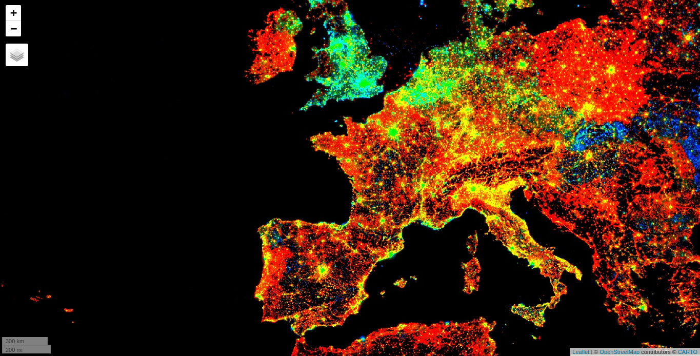
1. Compute the trend of night-time lights (JS version)

Authenticate and Initialize the Earth Engine R API.

library(rgee)
ee_Initialize()

Let’s create a new band containing the image date as years since 1991 by extracting the year of the image acquisition date and subtracting it from 1991.

createTimeBand <-function(img) {
  year <- ee$Date(img$get('system:time_start'))$get('year')$subtract(1991L) 
  ee$Image(year)$byte()$addBands(img)
}

Use your TimeBand function to map it over the night-time lights collection.

collection <- ee$
  ImageCollection('NOAA/DMSP-OLS/NIGHTTIME_LIGHTS')$
  select('stable_lights')$
  map(createTimeBand)

Compute a linear fit over the series of values at each pixel, so that you can visualize the y-intercept as green, and the positive/negative slopes as red/blue.

col_reduce <- collection$reduce(ee$Reducer$linearFit())
col_reduce <- col_reduce$addBands(
  col_reduce$select('scale'))
ee_print(col_reduce)

Let’s visualize our map!

Map$setCenter(9.08203, 47.39835, 3)
Map$addLayer(
  eeObject = col_reduce,
  visParams = list(
    bands = c("scale", "offset", "scale"),
    min = 0,
    max = c(0.18, 20, -0.18)
  ),
  name = "stable lights trend"
)

rgee_01

2. Let’s play with some precipitation values

Install and load tidyverse and sf R packages, and initialize the Earth Engine R API.

library(tidyverse)
library(rgee)
library(sf)

ee_Initialize()

Read the nc shapefile.

nc <- st_read(system.file("shape/nc.shp", package = "sf"), quiet = TRUE)

We will use the Terraclimate dataset to extract the monthly precipitation (Pr) from 2001

terraclimate <- ee$ImageCollection("IDAHO_EPSCOR/TERRACLIMATE") %>%
  ee$ImageCollection$filterDate("2001-01-01", "2002-01-01") %>%
  ee$ImageCollection$map(function(x) x$select("pr")) %>% # Select only precipitation bands
  ee$ImageCollection$toBands() %>% # from imagecollection to image
  ee$Image$rename(sprintf("PP_%02d",1:12)) # rename the bands of an image

ee_extract will help you to extract monthly precipitation values from the Terraclimate ImageCollection. ee_extract works similar to raster::extract, you just need to define: the ImageCollection object (x), the geometry (y), and a function to summarize the values (fun).

ee_nc_rain <- ee_extract(x = terraclimate, y = nc["NAME"], sf = FALSE)

Use ggplot2 to generate a beautiful static plot!

ee_nc_rain %>%
  pivot_longer(-NAME, names_to = "month", values_to = "pr") %>%
  mutate(month, month=gsub("PP_", "", month)) %>%
  ggplot(aes(x = month, y = pr, group = NAME, color = pr)) +
  geom_line(alpha = 0.4) +
  xlab("Month") +
  ylab("Precipitation (mm)") +
  theme_minimal()

### 3. Create an NDVI-animation (JS version)

Install and load sf. after that, initialize the Earth Engine R API.

library(magick)
library(rgee)
library(sf)

ee_Initialize()

Define the regional bounds of animation frames and a mask to clip the NDVI data by.

mask <- system.file("shp/arequipa.shp", package = "rgee") %>%
  st_read(quiet = TRUE) %>%
  sf_as_ee()
region <- mask$geometry()$bounds()

Retrieve the MODIS Terra Vegetation Indices 16-Day Global 1km dataset as an ee.ImageCollection and then, select the NDVI band.

col <- ee$ImageCollection('MODIS/006/MOD13A2')$select('NDVI')

Group images by composite date

col <- col$map(function(img) {
  doy <- ee$Date(img$get('system:time_start'))$getRelative('day', 'year')
  img$set('doy', doy)
})
distinctDOY <- col$filterDate('2013-01-01', '2014-01-01')

Now, let’s define a filter that identifies which images from the complete collection match the DOY from the distinct DOY collection.

filter <- ee$Filter$equals(leftField = 'doy', rightField = 'doy')

Define a join and convert the resulting FeatureCollection to an ImageCollection… it will take you only 2 lines of code!

join <- ee$Join$saveAll('doy_matches')
joinCol <- ee$ImageCollection(join$apply(distinctDOY, col, filter))

Apply median reduction among the matching DOY collections.

comp <- joinCol$map(function(img) {
  doyCol = ee$ImageCollection$fromImages(
    img$get('doy_matches')
  )
  doyCol$reduce(ee$Reducer$median())
})

Almost ready! but let’s define RGB visualization parameters first.

visParams = list(
  min = 0.0,
  max = 9000.0,
  bands = "NDVI_median",
  palette = c(
    'FFFFFF', 'CE7E45', 'DF923D', 'F1B555', 'FCD163', '99B718', '74A901',
    '66A000', '529400', '3E8601', '207401', '056201', '004C00', '023B01',
    '012E01', '011D01', '011301'
  )
)

Create RGB visualization images for use as animation frames.

rgbVis <- comp$map(function(img) {
  do.call(img$visualize, visParams) %>%
    ee$Image$clip(mask)
})

Let’s animate this. Define GIF visualization parameters.

gifParams <- list(
  region = region,
  dimensions = 600,
  crs = 'EPSG:3857',
  framesPerSecond = 10
)

Get month names

dates_modis_mabbr <- distinctDOY %>%
  ee_get_date_ic %>% # Get Image Collection dates
  '[['("time_start") %>% # Select time_start column
  lubridate::month() %>% # Get the month component of the datetime
  '['(month.abb, .) # subset around month abbreviations

And finally, use ee_utils_gif_* functions to render the GIF animation and add some texts.

animation <- ee_utils_gif_creator(rgbVis, gifParams, mode = "wb")
animation %>%
  ee_utils_gif_annotate(
    text = "NDVI: MODIS/006/MOD13A2",
    size = 15, color = "white",
    location = "+10+10"
  ) %>%
  ee_utils_gif_annotate(
    text = dates_modis_mabbr,
    size = 30,
    location = "+290+350",
    color = "white",
    font = "arial",
    boxcolor = "#000000"
  ) # -> animation_wtxt

# ee_utils_gif_save(animation_wtxt, path = "raster_as_ee.gif")

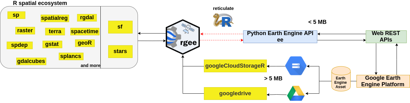
## How does rgee work?

rgee is not a native Earth Engine API like the Javascript or Python client. Developing an Earth Engine API from scratch would create too much maintenance burden, especially considering that the API is in active development. So, how is it possible to run Earth Engine using R? the answer is [reticulate]! (https://rstudio.github.io/reticulate/). reticulate is an R package designed to allow seamless interoperability between R and Python. When an Earth Engine request is created in R, reticulate will translate this request into Python and pass it to the Earth Engine Python API, which converts the request to a JSON format. Finally, the request is received by the GEE Platform through a Web REST API. The response will follow the same path in reverse.

workflow

Code of Conduct

Please note that the rgee project is released with a Contributor Code of Conduct. By contributing to this project, you agree to abide by its terms.

Contributing Guide

👍 Thanks for taking the time to contribute! 🎉👍 Please review our Contributing Guide.

Enjoying rgee? Let others know about it! Share it on Twitter, LinkedIN or in a blog post to spread the word.

Using rgee for your scientific article? here’s how you can cite it

citation("rgee")
To cite rgee in publications use:

  C Aybar, Q Wu, L Bautista, R Yali and A Barja (2020) rgee: An R
  package for interacting with Google Earth Engine Journal of Open
  Source Software URL https://github.com/r-spatial/rgee/.

A BibTeX entry for LaTeX users is

@Article{,
  title = {rgee: An R package for interacting with Google Earth Engine},
  author = {Cesar Aybar and Quisheng Wu and Lesly Bautista and Roy Yali and Antony Barja},
  journal = {Journal of Open Source Software},
  year = {2020},
}

Credits

We want to offer a special thanks 🙌 👏 to Justin Braaten for his wise and helpful comments in the whole development of rgee. As well, we would like to mention the following third-party R/Python packages for contributing indirectly to the improvement of rgee:

rgee: Google Earth Engine for R

rgee is an R binding package for calling Google Earth Engine API from within R. Various functions are implemented to simplify the connection with the R spatial ecosystem.

What is Google Earth Engine?

How to use

Installation

Sync rgee with other Python packages

Package Conventions

Hello World

1. Compute the trend of night-time lights (JS version)

2. Let’s play with some precipitation values

Code of Conduct

Contributing Guide

Credits

Links

License

Community

Citation

Developers

Dev status

rgee: Google Earth Engine for R

rgee is an R binding package for calling Google Earth Engine API from within R. Various functions are implemented to simplify the connection with the R spatial ecosystem.

What is Google Earth Engine?

How to use

Installation

Sync rgee with other Python packages

Package Conventions

Hello World

1. Compute the trend of night-time lights (JS version)

2. Let’s play with some precipitation values

Code of Conduct

Contributing Guide

Share the love

Credits

Links

License

Community

Citation

Developers

Dev status