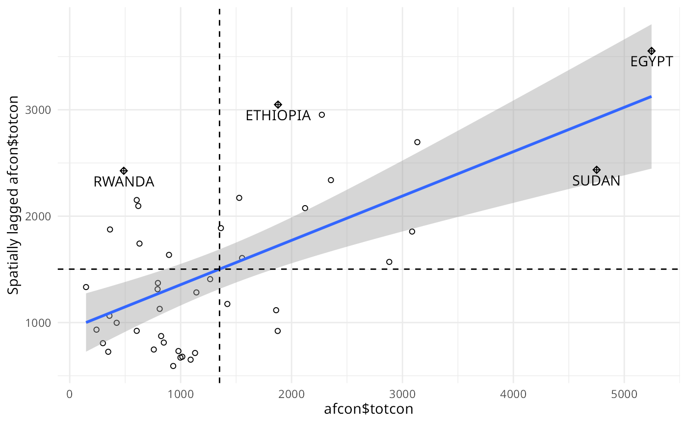
Moran scatterplot

A plot of spatial data against its spatially lagged values, augmented by reporting the summary of influence measures for the linear relationship between the data and the lag. If zero policy is TRUE, such observations are also marked if they occur.

Usage

moran.plot(x, listw, y=NULL, zero.policy=attr(listw, "zero.policy"), spChk=NULL,
 labels=NULL, xlab=NULL, ylab=NULL, quiet=NULL, plot=TRUE, return_df=TRUE, ...)

Arguments

x: a numeric vector the same length as the neighbours list in listw
listw: a listw object created for example by nb2listw
y: an optional numeric vector the same length as the neighbours list in listw for a bi-variate plot
zero.policy: default attr(listw, "zero.policy") as set when listw was created, if attribute not set, use global option value; if TRUE assign zero to the lagged value of zones without neighbours, if FALSE assign NA
spChk: should the data vector names be checked against the spatial objects for identity integrity, TRUE, or FALSE, default NULL to use get.spChkOption()
labels: character labels for points with high influence measures, if set to FALSE, no labels are plotted for points with large influence
xlab: label for x axis
ylab: label for x axis
quiet: default NULL, use !verbose global option value; if TRUE, output of summary of influence object suppressed
plot: default TRUE, if false, plotting is suppressed
return_df: default TRUE, invisibly return a data.frame object; if FALSE invisibly return an influence measures object
...: further graphical parameters as in par(..)

Value

The function returns a data.frame object with coordinates and influence measures if return_df is TRUE, or an influence object from influence.measures.

References

Anselin, L. 1996. The Moran scatterplot as an ESDA tool to assess local instability in spatial association. pp. 111–125 in M. M. Fischer, H. J. Scholten and D. Unwin (eds) Spatial analytical perspectives on GIS, London, Taylor and Francis; Anselin, L. 1995. Local indicators of spatial association, Geographical Analysis, 27, 93–115

Author

Roger Bivand Roger.Bivand@nhh.no

Examples

data(afcon, package="spData")
mp <- moran.plot(afcon$totcon, nb2listw(paper.nb),
 labels=as.character(afcon$name), pch=19)

moran.plot(as.vector(scale(afcon$totcon)), nb2listw(paper.nb),
 labels=as.character(afcon$name), xlim=c(-2, 4), ylim=c(-2,4), pch=19)

if (require(ggplot2, quietly=TRUE)) {
  xname <- attr(mp, "xname")
  ggplot(mp, aes(x=x, y=wx)) + geom_point(shape=1) + 
    geom_smooth(formula=y ~ x, method="lm") + 
    geom_hline(yintercept=mean(mp$wx), lty=2) + 
    geom_vline(xintercept=mean(mp$x), lty=2) + theme_minimal() + 
    geom_point(data=mp[mp$is_inf,], aes(x=x, y=wx), shape=9) +
    geom_text(data=mp[mp$is_inf,], aes(x=x, y=wx, label=labels, vjust=1.5)) +
    xlab(xname) + ylab(paste0("Spatially lagged ", xname))
}

columbus <- st_read(system.file("shapes/columbus.gpkg", package="spData"))
#> Reading layer `columbus' from data source 
#>   `/home/rsb/lib/r_libs/spData/shapes/columbus.gpkg' using driver `GPKG'
#> Simple feature collection with 49 features and 20 fields
#> Geometry type: POLYGON
#> Dimension:     XY
#> Bounding box:  xmin: 5.874907 ymin: 10.78863 xmax: 11.28742 ymax: 14.74245
#> Projected CRS: Undefined Cartesian SRS with unknown unit
nb <- poly2nb(columbus)
listw <- nb2listw(nb)
moran.plot(x=columbus$CRIME, y=columbus$INC, listw=listw)

moran.plot(x=columbus$INC, y=columbus$CRIME, listw=listw)