Neighbourhood contiguity by distance
dnearneigh.RdThe function identifies neighbours of region points by Euclidean distance in the metric of the points between lower (greater than or equal to (changed from version 1.1-7)) and upper (less than or equal to) bounds, or with longlat = TRUE, by Great Circle distance in kilometers. If x is an "sf" object and use_s2= is TRUE, spherical distances in km are used.
Usage
dnearneigh(x, d1, d2, row.names = NULL, longlat = NULL, bounds=c("GE", "LE"),
 use_kd_tree=TRUE, symtest=FALSE, use_s2=packageVersion("s2") > "1.0.7", k=200,
 dwithin=TRUE)
Arguments
- x
matrix of point coordinates, an object inheriting from SpatialPoints or an
"sf"or"sfc"object; if the"sf"or"sfc"object geometries are in geographical coordinates (use_s2=FALSE,sf::st_is_longlat(x) == TRUEandsf::sf_use_s2() == TRUE), s2 will be used to find the neighbours because it will (we hope) use spatial indexing https://github.com/r-spatial/s2/issues/125 as opposed to the legacy method which uses brute-force (at present s2 also uses brute-force)- d1
lower distance bound in the metric of the points if planar coordinates, in km if in geographical coordinates
- d2
upper distance boundd in the metric of the points if planar coordinates, in km if in geographical coordinates
- row.names
character vector of region ids to be added to the neighbours list as attribute
region.id, defaultseq(1, nrow(x))- longlat
TRUE if point coordinates are geographical longitude-latitude decimal degrees, in which case distances are measured in kilometers; if x is a SpatialPoints object, the value is taken from the object itself, and overrides this argument if not NULL
- bounds
character vector of length 2, default
c("GE", "LE"), (GE: greater than or equal to, LE: less than or equal to) that is the finite and closed interval[d1, d2],d1 <= x <= d2. The first element may also be"GT"(GT: greater than), the second"LT"(LT: less than) for finite, open intervals excluding the bounds; the first bound default was changed from"GT"to"GE"in release 1.1-7. When creating multiple distance bands, finite, half-open right-closed intervals may be used until the final interval to avoid overlapping on bounds:"GE", "LT", that is[d1, d2),d1 <= x < d2- use_kd_tree
default TRUE, if TRUE, use dbscan
frNNif available (permitting 3D distances).- symtest
Default FALSE; before release 1.1-7, TRUE - run symmetry check on output object, costly with large numbers of points.
- use_s2
default=
packageVersion("s2") > "1.0.7", as of s2 > 1.0-7, distance bound computations use spatial indexing so whensf::sf_use_s2()is TRUE,s2::s2_dwithin_matrix()will be used for distances on the sphere for"sf"or"sfc"objects if s2 > 1.0-7.- k
default 200, the number of closest points to consider when searching when using
s2::s2_closest_edges()- dwithin
default TRUE, if FALSE, use
s2::s2_closest_edges(), both ifuse_s2=TRUE,sf::st_is_longlat(x) == TRUEandsf::sf_use_s2() == TRUE;s2::s2_dwithin_matrix()yields the same lists of neighbours ass2::s2_closest_edges()isk=is set correctly.
Value
The function returns a list of integer vectors giving the region id numbers
for neighbours satisfying the distance criteria. See card for details of “nb” objects.
Author
Roger Bivand Roger.Bivand@nhh.no
Examples
columbus <- st_read(system.file("shapes/columbus.gpkg", package="spData")[1], quiet=TRUE)
coords <- st_centroid(st_geometry(columbus), of_largest_polygon=TRUE)
rn <- row.names(columbus)
k1 <- knn2nb(knearneigh(coords))
#> Warning: neighbour object has 13 sub-graphs
all.linked <- max(unlist(nbdists(k1, coords)))
col.nb.0.all <- dnearneigh(coords, 0, all.linked, row.names=rn)
#> Warning: neighbour object has 2 sub-graphs
summary(col.nb.0.all, coords)
#> Neighbour list object:
#> Number of regions: 49
#> Number of nonzero links: 252
#> Percentage nonzero weights: 10.49563
#> Average number of links: 5.142857
#> 2 disjoint connected subgraphs
#> Link number distribution:
#>
#> 1 2 3 4 5 6 7 8 9 10 11
#> 4 8 6 2 5 8 6 2 6 1 1
#> 4 least connected regions:
#> 6 10 21 47 with 1 link
#> 1 most connected region:
#> 28 with 11 links
opar <- par(no.readonly=TRUE)
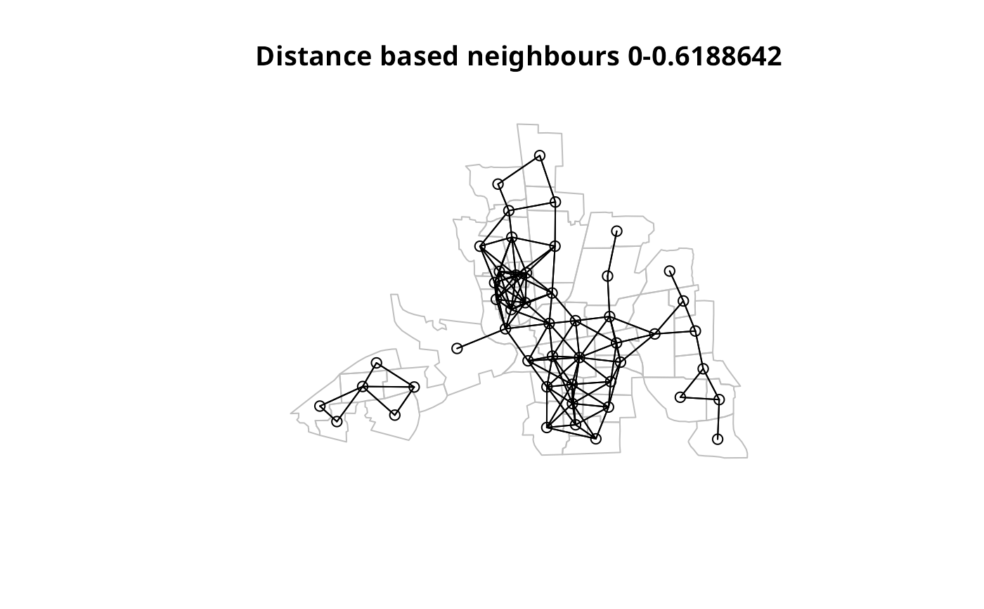
plot(st_geometry(columbus), border="grey", reset=FALSE,
main=paste("Distance based neighbours 0-", format(all.linked), sep=""))
plot(col.nb.0.all, coords, add=TRUE)
 par(opar)
(sfc_obj <- st_centroid(st_geometry(columbus)))
#> Geometry set for 49 features
#> Geometry type: POINT
#> Dimension: XY
#> Bounding box: xmin: 6.221943 ymin: 11.01003 xmax: 10.95359 ymax: 14.36908
#> Projected CRS: Undefined Cartesian SRS with unknown unit
#> First 5 geometries:
#> POINT (8.827218 14.36908)
#> POINT (8.332658 14.03162)
#> POINT (9.012265 13.81972)
#> POINT (8.460801 13.71696)
#> POINT (9.007982 13.29637)
col.nb.0.all_sf <- dnearneigh(sfc_obj, 0, all.linked, row.names=rn)
#> Warning: neighbour object has 2 sub-graphs
all.equal(col.nb.0.all, col.nb.0.all_sf, check.attributes=FALSE)
#> [1] TRUE
data(state)
us48.fipsno <- read.geoda(system.file("etc/weights/us48.txt",
package="spdep")[1])
if (as.numeric(paste(version$major, version$minor, sep="")) < 19) {
m50.48 <- match(us48.fipsno$"State.name", state.name)
} else {
m50.48 <- match(us48.fipsno$"State_name", state.name)
}
xy <- as.matrix(as.data.frame(state.center))[m50.48,]
llk1 <- knn2nb(knearneigh(xy, k=1, longlat=FALSE))
#> Warning: neighbour object has 12 sub-graphs
(all.linked <- max(unlist(nbdists(llk1, xy, longlat=FALSE))))
#> [1] 5.161223
ll.nb <- dnearneigh(xy, 0, all.linked, longlat=FALSE)
#> Warning: neighbour object has 5 sub-graphs
summary(ll.nb, xy, longlat=TRUE, scale=0.5)
#> Neighbour list object:
#> Number of regions: 48
#> Number of nonzero links: 190
#> Percentage nonzero weights: 8.246528
#> Average number of links: 3.958333
#> 5 disjoint connected subgraphs
#> Link number distribution:
#>
#> 1 2 3 4 5 7 8 9 10
#> 11 9 4 8 4 4 4 3 1
#> 11 least connected regions:
#> 2 4 8 10 24 26 29 32 35 41 45 with 1 link
#> 1 most connected region:
#> 28 with 10 links
gck1 <- knn2nb(knearneigh(xy, k=1, longlat=TRUE))
#> Warning: neighbour object has 11 sub-graphs
(all.linked <- max(unlist(nbdists(gck1, xy, longlat=TRUE))))
#> [1] 523.5819
gc.nb <- dnearneigh(xy, 0, all.linked, longlat=TRUE)
#> Warning: neighbour object has 2 sub-graphs
summary(gc.nb, xy, longlat=TRUE, scale=0.5)
#> Neighbour list object:
#> Number of regions: 48
#> Number of nonzero links: 220
#> Percentage nonzero weights: 9.548611
#> Average number of links: 4.583333
#> 2 disjoint connected subgraphs
#> Link number distribution:
#>
#> 1 2 3 4 5 6 7 8 9 10
#> 5 9 6 8 5 2 3 3 5 2
#> 5 least connected regions:
#> 2 4 8 41 45 with 1 link
#> 2 most connected regions:
#> 7 28 with 10 links
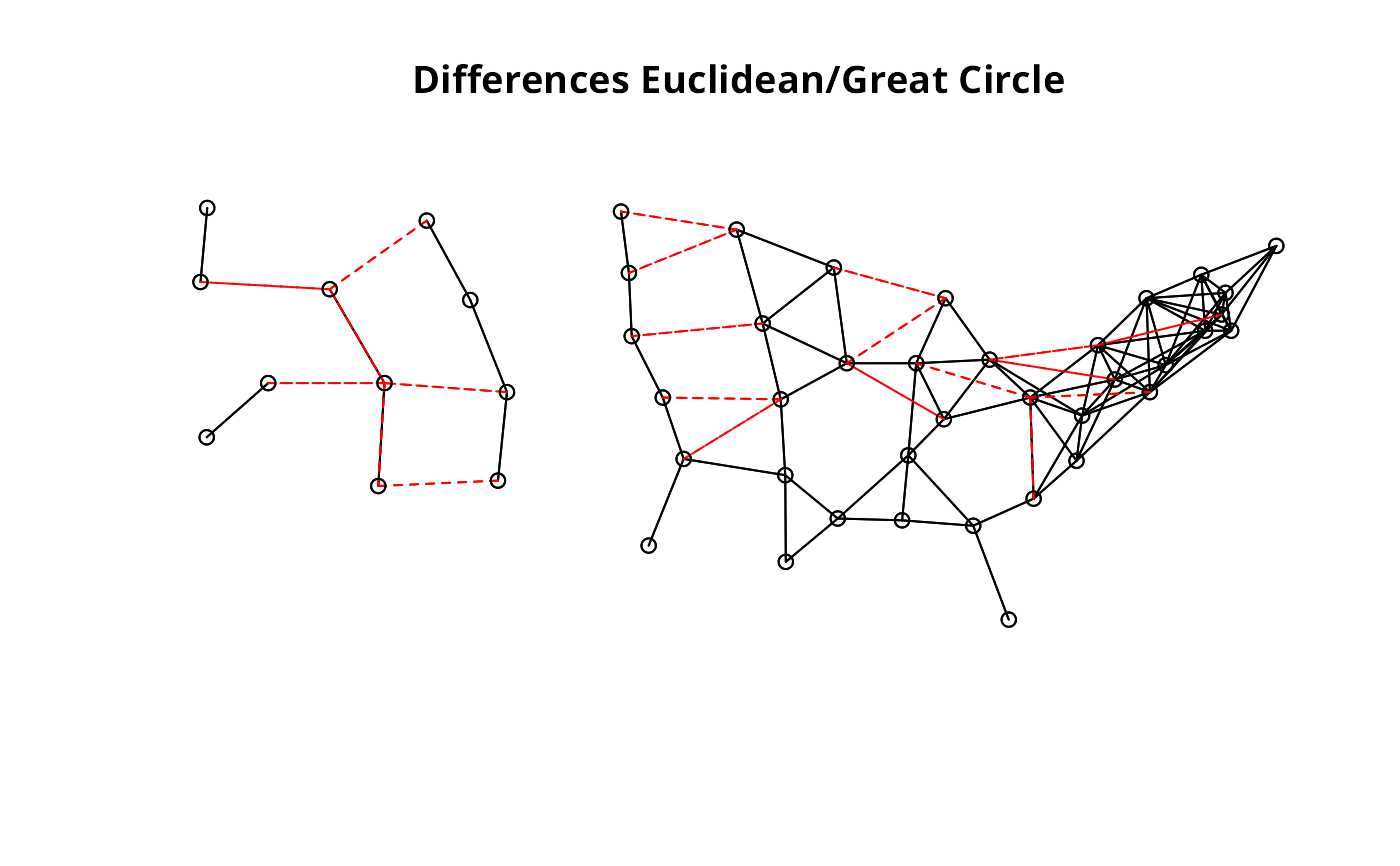
plot(ll.nb, xy)
plot(diffnb(ll.nb, gc.nb), xy, add=TRUE, col="red", lty=2)
#> Warning: neighbour object has 27 sub-graphs
title(main="Differences Euclidean/Great Circle")
par(opar)
(sfc_obj <- st_centroid(st_geometry(columbus)))
#> Geometry set for 49 features
#> Geometry type: POINT
#> Dimension: XY
#> Bounding box: xmin: 6.221943 ymin: 11.01003 xmax: 10.95359 ymax: 14.36908
#> Projected CRS: Undefined Cartesian SRS with unknown unit
#> First 5 geometries:
#> POINT (8.827218 14.36908)
#> POINT (8.332658 14.03162)
#> POINT (9.012265 13.81972)
#> POINT (8.460801 13.71696)
#> POINT (9.007982 13.29637)
col.nb.0.all_sf <- dnearneigh(sfc_obj, 0, all.linked, row.names=rn)
#> Warning: neighbour object has 2 sub-graphs
all.equal(col.nb.0.all, col.nb.0.all_sf, check.attributes=FALSE)
#> [1] TRUE
data(state)
us48.fipsno <- read.geoda(system.file("etc/weights/us48.txt",
package="spdep")[1])
if (as.numeric(paste(version$major, version$minor, sep="")) < 19) {
m50.48 <- match(us48.fipsno$"State.name", state.name)
} else {
m50.48 <- match(us48.fipsno$"State_name", state.name)
}
xy <- as.matrix(as.data.frame(state.center))[m50.48,]
llk1 <- knn2nb(knearneigh(xy, k=1, longlat=FALSE))
#> Warning: neighbour object has 12 sub-graphs
(all.linked <- max(unlist(nbdists(llk1, xy, longlat=FALSE))))
#> [1] 5.161223
ll.nb <- dnearneigh(xy, 0, all.linked, longlat=FALSE)
#> Warning: neighbour object has 5 sub-graphs
summary(ll.nb, xy, longlat=TRUE, scale=0.5)
#> Neighbour list object:
#> Number of regions: 48
#> Number of nonzero links: 190
#> Percentage nonzero weights: 8.246528
#> Average number of links: 3.958333
#> 5 disjoint connected subgraphs
#> Link number distribution:
#>
#> 1 2 3 4 5 7 8 9 10
#> 11 9 4 8 4 4 4 3 1
#> 11 least connected regions:
#> 2 4 8 10 24 26 29 32 35 41 45 with 1 link
#> 1 most connected region:
#> 28 with 10 links
gck1 <- knn2nb(knearneigh(xy, k=1, longlat=TRUE))
#> Warning: neighbour object has 11 sub-graphs
(all.linked <- max(unlist(nbdists(gck1, xy, longlat=TRUE))))
#> [1] 523.5819
gc.nb <- dnearneigh(xy, 0, all.linked, longlat=TRUE)
#> Warning: neighbour object has 2 sub-graphs
summary(gc.nb, xy, longlat=TRUE, scale=0.5)
#> Neighbour list object:
#> Number of regions: 48
#> Number of nonzero links: 220
#> Percentage nonzero weights: 9.548611
#> Average number of links: 4.583333
#> 2 disjoint connected subgraphs
#> Link number distribution:
#>
#> 1 2 3 4 5 6 7 8 9 10
#> 5 9 6 8 5 2 3 3 5 2
#> 5 least connected regions:
#> 2 4 8 41 45 with 1 link
#> 2 most connected regions:
#> 7 28 with 10 links
plot(ll.nb, xy)
plot(diffnb(ll.nb, gc.nb), xy, add=TRUE, col="red", lty=2)
#> Warning: neighbour object has 27 sub-graphs
title(main="Differences Euclidean/Great Circle")
 #xy1 <- SpatialPoints((as.data.frame(state.center))[m50.48,],
# proj4string=CRS("+proj=longlat +ellps=GRS80"))
#gck1a <- knn2nb(knearneigh(xy1, k=1))
#(all.linked <- max(unlist(nbdists(gck1a, xy1))))
#gc.nb <- dnearneigh(xy1, 0, all.linked)
#summary(gc.nb, xy1, scale=0.5)
xy1 <- st_as_sf((as.data.frame(state.center))[m50.48,], coords=1:2,
crs=st_crs("OGC:CRS84"))
old_use_s2 <- sf_use_s2()
sf_use_s2(TRUE)
gck1b <- knn2nb(knearneigh(xy1, k=1))
#> Warning: neighbour object has 11 sub-graphs
system.time(o <- nbdists(gck1b, xy1))
#> user system elapsed
#> 0.006 0.000 0.006
(all.linked <- max(unlist(o)))
#> [1] 522.4464
# use s2 brute-force dwithin_matrix approach for s2 <= 1.0.7
system.time(gc.nb.dwithin <- dnearneigh(xy1, 0, all.linked, use_s2=TRUE, dwithin=TRUE))
#> Warning: neighbour object has 3 sub-graphs
#> user system elapsed
#> 0.011 0.001 0.012
summary(gc.nb, xy1, scale=0.5)
#> Neighbour list object:
#> Number of regions: 48
#> Number of nonzero links: 220
#> Percentage nonzero weights: 9.548611
#> Average number of links: 4.583333
#> 2 disjoint connected subgraphs
#> Link number distribution:
#>
#> 1 2 3 4 5 6 7 8 9 10
#> 5 9 6 8 5 2 3 3 5 2
#> 5 least connected regions:
#> 2 4 8 41 45 with 1 link
#> 2 most connected regions:
#> 7 28 with 10 links
# use s2 closest_edges approach s2 > 1.0.7
if (packageVersion("s2") > "1.0.7") {
(system.time(gc.nb.closest <- dnearneigh(xy1, 0, all.linked, dwithin=FALSE)))
}
#> Warning: neighbour object has 3 sub-graphs
#> user system elapsed
#> 0.010 0.000 0.011
if (packageVersion("s2") > "1.0.7") {
system.time(gc.nb.dwithin <- dnearneigh(xy1, 0, all.linked, use_s2=TRUE, dwithin=TRUE))
}
#> Warning: neighbour object has 3 sub-graphs
#> user system elapsed
#> 0.012 0.000 0.012
if (packageVersion("s2") > "1.0.7") {
summary(gc.nb.dwithin, xy1, scale=0.5)
}
#> Neighbour list object:
#> Number of regions: 48
#> Number of nonzero links: 218
#> Percentage nonzero weights: 9.461806
#> Average number of links: 4.541667
#> 1 region with no links:
#> 2
#> 3 disjoint connected subgraphs
#> Link number distribution:
#>
#> 0 1 2 3 4 5 6 7 8 9 10
#> 1 5 8 6 8 5 2 3 3 5 2
#> 5 least connected regions:
#> 4 8 29 41 45 with 1 link
#> 2 most connected regions:
#> 7 28 with 10 links
if (packageVersion("s2") > "1.0.7") {
summary(gc.nb.closest, xy1, scale=0.5)
}
#> Neighbour list object:
#> Number of regions: 48
#> Number of nonzero links: 218
#> Percentage nonzero weights: 9.461806
#> Average number of links: 4.541667
#> 1 region with no links:
#> 2
#> 3 disjoint connected subgraphs
#> Link number distribution:
#>
#> 0 1 2 3 4 5 6 7 8 9 10
#> 1 5 8 6 8 5 2 3 3 5 2
#> 5 least connected regions:
#> 4 8 29 41 45 with 1 link
#> 2 most connected regions:
#> 7 28 with 10 links
# use legacy symmetric brute-force approach
system.time(gc.nb.legacy <- dnearneigh(xy1, 0, all.linked, use_s2=FALSE))
#> Warning: neighbour object has 3 sub-graphs
#> user system elapsed
#> 0.007 0.000 0.006
summary(gc.nb, xy1, scale=0.5)
#> Neighbour list object:
#> Number of regions: 48
#> Number of nonzero links: 220
#> Percentage nonzero weights: 9.548611
#> Average number of links: 4.583333
#> 2 disjoint connected subgraphs
#> Link number distribution:
#>
#> 1 2 3 4 5 6 7 8 9 10
#> 5 9 6 8 5 2 3 3 5 2
#> 5 least connected regions:
#> 2 4 8 41 45 with 1 link
#> 2 most connected regions:
#> 7 28 with 10 links
if (packageVersion("s2") > "1.0.7") all.equal(gc.nb.closest, gc.nb.dwithin, check.attributes=FALSE)
#> [1] TRUE
# legacy is ellipsoidal, s2 spherical, so minor differences expected
if (packageVersion("s2") > "1.0.7") all.equal(gc.nb, gc.nb.closest, check.attributes=FALSE)
#> [1] "Component 2: Mean relative difference: 1"
#> [2] "Component 29: Numeric: lengths (2, 1) differ"
all.equal(gc.nb, gc.nb.dwithin, check.attributes=FALSE)
#> [1] "Component 2: Mean relative difference: 1"
#> [2] "Component 29: Numeric: lengths (2, 1) differ"
sf_use_s2(old_use_s2)
# example of reading points with readr::read_csv() yielding a tibble
load(system.file("etc/misc/coords.rda", package="spdep"))
class(coords)
#> [1] "spec_tbl_df" "tbl_df" "tbl" "data.frame"
k1 <- knn2nb(knearneigh(coords, k=1))
#> Warning: neighbour object has 29 sub-graphs
all.linked <- max(unlist(nbdists(k1, coords)))
dnearneigh(coords, 0, all.linked)
#> Neighbour list object:
#> Number of regions: 100
#> Number of nonzero links: 676
#> Percentage nonzero weights: 6.76
#> Average number of links: 6.76
#xy1 <- SpatialPoints((as.data.frame(state.center))[m50.48,],
# proj4string=CRS("+proj=longlat +ellps=GRS80"))
#gck1a <- knn2nb(knearneigh(xy1, k=1))
#(all.linked <- max(unlist(nbdists(gck1a, xy1))))
#gc.nb <- dnearneigh(xy1, 0, all.linked)
#summary(gc.nb, xy1, scale=0.5)
xy1 <- st_as_sf((as.data.frame(state.center))[m50.48,], coords=1:2,
crs=st_crs("OGC:CRS84"))
old_use_s2 <- sf_use_s2()
sf_use_s2(TRUE)
gck1b <- knn2nb(knearneigh(xy1, k=1))
#> Warning: neighbour object has 11 sub-graphs
system.time(o <- nbdists(gck1b, xy1))
#> user system elapsed
#> 0.006 0.000 0.006
(all.linked <- max(unlist(o)))
#> [1] 522.4464
# use s2 brute-force dwithin_matrix approach for s2 <= 1.0.7
system.time(gc.nb.dwithin <- dnearneigh(xy1, 0, all.linked, use_s2=TRUE, dwithin=TRUE))
#> Warning: neighbour object has 3 sub-graphs
#> user system elapsed
#> 0.011 0.001 0.012
summary(gc.nb, xy1, scale=0.5)
#> Neighbour list object:
#> Number of regions: 48
#> Number of nonzero links: 220
#> Percentage nonzero weights: 9.548611
#> Average number of links: 4.583333
#> 2 disjoint connected subgraphs
#> Link number distribution:
#>
#> 1 2 3 4 5 6 7 8 9 10
#> 5 9 6 8 5 2 3 3 5 2
#> 5 least connected regions:
#> 2 4 8 41 45 with 1 link
#> 2 most connected regions:
#> 7 28 with 10 links
# use s2 closest_edges approach s2 > 1.0.7
if (packageVersion("s2") > "1.0.7") {
(system.time(gc.nb.closest <- dnearneigh(xy1, 0, all.linked, dwithin=FALSE)))
}
#> Warning: neighbour object has 3 sub-graphs
#> user system elapsed
#> 0.010 0.000 0.011
if (packageVersion("s2") > "1.0.7") {
system.time(gc.nb.dwithin <- dnearneigh(xy1, 0, all.linked, use_s2=TRUE, dwithin=TRUE))
}
#> Warning: neighbour object has 3 sub-graphs
#> user system elapsed
#> 0.012 0.000 0.012
if (packageVersion("s2") > "1.0.7") {
summary(gc.nb.dwithin, xy1, scale=0.5)
}
#> Neighbour list object:
#> Number of regions: 48
#> Number of nonzero links: 218
#> Percentage nonzero weights: 9.461806
#> Average number of links: 4.541667
#> 1 region with no links:
#> 2
#> 3 disjoint connected subgraphs
#> Link number distribution:
#>
#> 0 1 2 3 4 5 6 7 8 9 10
#> 1 5 8 6 8 5 2 3 3 5 2
#> 5 least connected regions:
#> 4 8 29 41 45 with 1 link
#> 2 most connected regions:
#> 7 28 with 10 links
if (packageVersion("s2") > "1.0.7") {
summary(gc.nb.closest, xy1, scale=0.5)
}
#> Neighbour list object:
#> Number of regions: 48
#> Number of nonzero links: 218
#> Percentage nonzero weights: 9.461806
#> Average number of links: 4.541667
#> 1 region with no links:
#> 2
#> 3 disjoint connected subgraphs
#> Link number distribution:
#>
#> 0 1 2 3 4 5 6 7 8 9 10
#> 1 5 8 6 8 5 2 3 3 5 2
#> 5 least connected regions:
#> 4 8 29 41 45 with 1 link
#> 2 most connected regions:
#> 7 28 with 10 links
# use legacy symmetric brute-force approach
system.time(gc.nb.legacy <- dnearneigh(xy1, 0, all.linked, use_s2=FALSE))
#> Warning: neighbour object has 3 sub-graphs
#> user system elapsed
#> 0.007 0.000 0.006
summary(gc.nb, xy1, scale=0.5)
#> Neighbour list object:
#> Number of regions: 48
#> Number of nonzero links: 220
#> Percentage nonzero weights: 9.548611
#> Average number of links: 4.583333
#> 2 disjoint connected subgraphs
#> Link number distribution:
#>
#> 1 2 3 4 5 6 7 8 9 10
#> 5 9 6 8 5 2 3 3 5 2
#> 5 least connected regions:
#> 2 4 8 41 45 with 1 link
#> 2 most connected regions:
#> 7 28 with 10 links
if (packageVersion("s2") > "1.0.7") all.equal(gc.nb.closest, gc.nb.dwithin, check.attributes=FALSE)
#> [1] TRUE
# legacy is ellipsoidal, s2 spherical, so minor differences expected
if (packageVersion("s2") > "1.0.7") all.equal(gc.nb, gc.nb.closest, check.attributes=FALSE)
#> [1] "Component 2: Mean relative difference: 1"
#> [2] "Component 29: Numeric: lengths (2, 1) differ"
all.equal(gc.nb, gc.nb.dwithin, check.attributes=FALSE)
#> [1] "Component 2: Mean relative difference: 1"
#> [2] "Component 29: Numeric: lengths (2, 1) differ"
sf_use_s2(old_use_s2)
# example of reading points with readr::read_csv() yielding a tibble
load(system.file("etc/misc/coords.rda", package="spdep"))
class(coords)
#> [1] "spec_tbl_df" "tbl_df" "tbl" "data.frame"
k1 <- knn2nb(knearneigh(coords, k=1))
#> Warning: neighbour object has 29 sub-graphs
all.linked <- max(unlist(nbdists(k1, coords)))
dnearneigh(coords, 0, all.linked)
#> Neighbour list object:
#> Number of regions: 100
#> Number of nonzero links: 676
#> Percentage nonzero weights: 6.76
#> Average number of links: 6.76