K nearest neighbours for spatial weights

The function returns a matrix with the indices of points belonging to the set of the k nearest neighbours of each other. If longlat = TRUE, Great Circle distances are used. A warning will be given if identical points are found.

knearneigh(x, k=1, longlat = NULL, use_kd_tree=TRUE)

Arguments

x

matrix of point coordinates, an object inheriting from SpatialPoints or an "sf" or "sfc" object; if the "sf" or "sfc" object geometries are in geographical coordinates (sf::st_is_longlat(x) == TRUE and sf::sf_use_s2() == TRUE), s2 will be used to find the neighbours because it uses spatial indexing https://github.com/r-spatial/s2/issues/125 as opposed to the legacy method which uses brute-force

k

number of nearest neighbours to be returned

longlat

TRUE if point coordinates are longitude-latitude decimal degrees, in which case distances are measured in kilometers; if x is a SpatialPoints object, the value is taken from the object itself; longlat will override kd_tree

use_kd_tree

logical value, if the dbscan package is available, use for finding k nearest neighbours when longlat is FALSE, and when there are no identical points; from https://github.com/r-spatial/spdep/issues/38, the input data may have more than two columns if dbscan is used

Details

The underlying legacy C code is based on the knn function in the class package.

Value

A list of class knn

nn

integer matrix of region number ids

np

number of input points

k

input required k

dimension

number of columns of x

x

input coordinates

Author

Roger Bivand Roger.Bivand@nhh.no

See also

knn, dnearneigh, knn2nb, kNN

Examples

columbus <- st_read(system.file("shapes/columbus.shp", package="spData")[1], quiet=TRUE)
coords <- st_centroid(st_geometry(columbus), of_largest_polygon=TRUE)
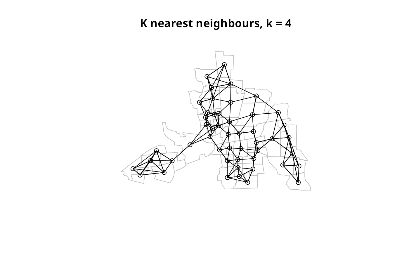
col.knn <- knearneigh(coords, k=4)
plot(st_geometry(columbus), border="grey")
plot(knn2nb(col.knn), coords, add=TRUE)
title(main="K nearest neighbours, k = 4")

data(state)
us48.fipsno <- read.geoda(system.file("etc/weights/us48.txt",
 package="spdep")[1])
if (as.numeric(paste(version$major, version$minor, sep="")) < 19) {
 m50.48 <- match(us48.fipsno$"State.name", state.name)
} else {
 m50.48 <- match(us48.fipsno$"State_name", state.name)
}
xy <- as.matrix(as.data.frame(state.center))[m50.48,]
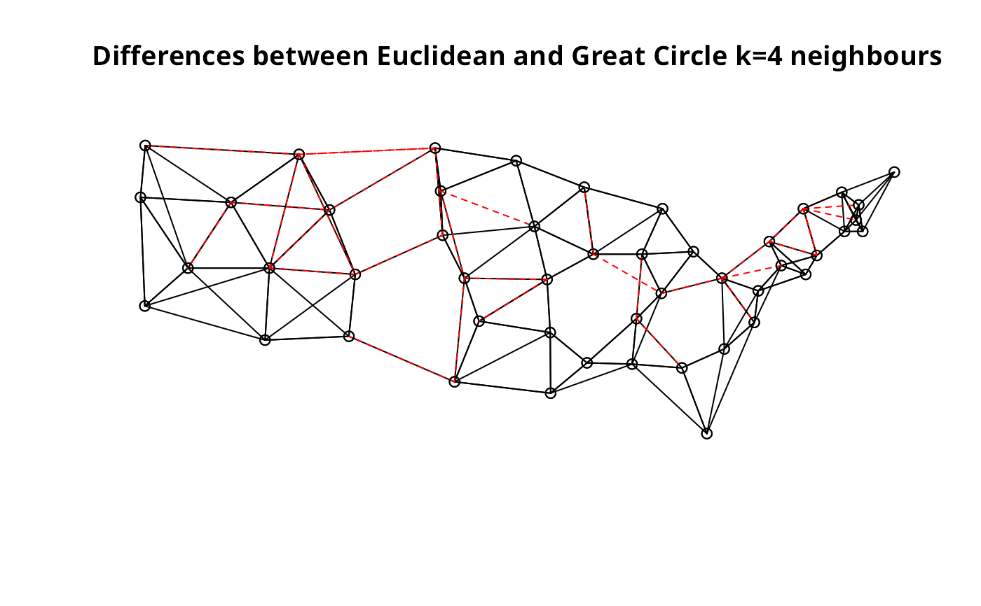
llk4.nb <- knn2nb(knearneigh(xy, k=4, longlat=FALSE))
gck4.nb <- knn2nb(knearneigh(xy, k=4, longlat=TRUE))
plot(llk4.nb, xy)
plot(diffnb(llk4.nb, gck4.nb), xy, add=TRUE, col="red", lty=2)
title(main="Differences between Euclidean and Great Circle k=4 neighbours")

summary(llk4.nb, xy, longlat=TRUE, scale=0.5)
#> Neighbour list object:
#> Number of regions: 48 
#> Number of nonzero links: 192 
#> Percentage nonzero weights: 8.333333 
#> Average number of links: 4 
#> Non-symmetric neighbours list
#> Link number distribution:
#> 
#>  4 
#> 48 
#> 48 least connected regions:
#> 1 2 3 4 5 6 7 8 9 10 11 12 13 14 15 16 17 18 19 20 21 22 23 24 25 26 27 28 29 30 31 32 33 34 35 36 37 38 39 40 41 42 43 44 45 46 47 48 with 4 links
#> 48 most connected regions:
#> 1 2 3 4 5 6 7 8 9 10 11 12 13 14 15 16 17 18 19 20 21 22 23 24 25 26 27 28 29 30 31 32 33 34 35 36 37 38 39 40 41 42 43 44 45 46 47 48 with 4 links
#> Summary of link distances:
#>    Min. 1st Qu.  Median    Mean 3rd Qu.    Max. 
#>   93.66  297.56  393.72  414.78  513.25  956.71 
#> 
#>   The decimal point is 2 digit(s) to the right of the |
#> 
#>   0 | 99
#>   1 | 00112233666699
#>   2 | 002222223344444444446677889999
#>   3 | 00000111112222222233333333334444556666777788899999
#>   4 | 0000001111233555555666666677788888899
#>   5 | 001111111112222222234444455666679
#>   6 | 002335667
#>   7 | 0112345889
#>   8 | 02279
#>   9 | 56
#> 
summary(gck4.nb, xy, longlat=TRUE, scale=0.5)
#> Neighbour list object:
#> Number of regions: 48 
#> Number of nonzero links: 192 
#> Percentage nonzero weights: 8.333333 
#> Average number of links: 4 
#> Non-symmetric neighbours list
#> Link number distribution:
#> 
#>  4 
#> 48 
#> 48 least connected regions:
#> 1 2 3 4 5 6 7 8 9 10 11 12 13 14 15 16 17 18 19 20 21 22 23 24 25 26 27 28 29 30 31 32 33 34 35 36 37 38 39 40 41 42 43 44 45 46 47 48 with 4 links
#> 48 most connected regions:
#> 1 2 3 4 5 6 7 8 9 10 11 12 13 14 15 16 17 18 19 20 21 22 23 24 25 26 27 28 29 30 31 32 33 34 35 36 37 38 39 40 41 42 43 44 45 46 47 48 with 4 links
#> Summary of link distances:
#>    Min. 1st Qu.  Median    Mean 3rd Qu.    Max. 
#>   93.66  297.09  393.72  410.42  508.50  953.23 
#> 
#>   The decimal point is 2 digit(s) to the right of the |
#> 
#>   0 | 99
#>   1 | 00112233666699
#>   2 | 0022222233444444444466778899999
#>   3 | 0000001111122222222333333333344445566677778888999
#>   4 | 00000011112335555556666666777788888899
#>   5 | 0001111111112222222344444456667899
#>   6 | 0023356
#>   7 | 000112455899
#>   8 | 0229
#>   9 | 5
#> 

xy1 <- SpatialPoints((as.data.frame(state.center))[m50.48,],
  proj4string=CRS("+proj=longlat +ellps=GRS80"))
gck4a.nb <- knn2nb(knearneigh(xy1, k=4))
summary(gck4a.nb, xy1, scale=0.5)
#> Neighbour list object:
#> Number of regions: 48 
#> Number of nonzero links: 192 
#> Percentage nonzero weights: 8.333333 
#> Average number of links: 4 
#> Non-symmetric neighbours list
#> Link number distribution:
#> 
#>  4 
#> 48 
#> 48 least connected regions:
#> 1 2 3 4 5 6 7 8 9 10 11 12 13 14 15 16 17 18 19 20 21 22 23 24 25 26 27 28 29 30 31 32 33 34 35 36 37 38 39 40 41 42 43 44 45 46 47 48 with 4 links
#> 48 most connected regions:
#> 1 2 3 4 5 6 7 8 9 10 11 12 13 14 15 16 17 18 19 20 21 22 23 24 25 26 27 28 29 30 31 32 33 34 35 36 37 38 39 40 41 42 43 44 45 46 47 48 with 4 links
#> Summary of link distances:
#>    Min. 1st Qu.  Median    Mean 3rd Qu.    Max. 
#>   93.66  297.09  393.72  410.42  508.50  953.23 
#> 
#>   The decimal point is 2 digit(s) to the right of the |
#> 
#>   0 | 99
#>   1 | 00112233666699
#>   2 | 0022222233444444444466778899999
#>   3 | 0000001111122222222333333333344445566677778888999
#>   4 | 00000011112335555556666666777788888899
#>   5 | 0001111111112222222344444456667899
#>   6 | 0023356
#>   7 | 000112455899
#>   8 | 0229
#>   9 | 5
#> 

xy1 <- st_as_sf((as.data.frame(state.center))[m50.48,], coords=1:2,
  crs=st_crs("+proj=longlat +ellps=GRS80"))
old_use_s2 <- sf_use_s2()
sf_use_s2(TRUE)
system.time(gck4a.nb <- knn2nb(knearneigh(xy1, k=4)))
#>    user  system elapsed 
#>   0.023   0.000   0.023 
summary(gck4a.nb, xy1, scale=0.5)
#> Neighbour list object:
#> Number of regions: 48 
#> Number of nonzero links: 192 
#> Percentage nonzero weights: 8.333333 
#> Average number of links: 4 
#> Non-symmetric neighbours list
#> Link number distribution:
#> 
#>  4 
#> 48 
#> 48 least connected regions:
#> 1 2 3 4 5 6 7 8 9 10 11 12 13 14 15 16 17 18 19 20 21 22 23 24 25 26 27 28 29 30 31 32 33 34 35 36 37 38 39 40 41 42 43 44 45 46 47 48 with 4 links
#> 48 most connected regions:
#> 1 2 3 4 5 6 7 8 9 10 11 12 13 14 15 16 17 18 19 20 21 22 23 24 25 26 27 28 29 30 31 32 33 34 35 36 37 38 39 40 41 42 43 44 45 46 47 48 with 4 links
#> Warning: number of items to replace is not a multiple of replacement length
#> Summary of link distances:
#>    Min. 1st Qu.  Median    Mean 3rd Qu.    Max. 
#>   102.5   296.6   409.3   421.1   527.8   820.3 
#> 
#>   The decimal point is 2 digit(s) to the right of the |
#> 
#>   0 | 01166
#>   2 | 24889900012223488
#>   4 | 00235661111122467888
#>   6 | 21248
#>   8 | 2
#> 
sf_use_s2(FALSE)
#> Spherical geometry (s2) switched off
system.time(gck4a.nb <- knn2nb(knearneigh(xy1, k=4)))
#>    user  system elapsed 
#>   0.011   0.000   0.011 
summary(gck4a.nb, xy1, scale=0.5)
#> Neighbour list object:
#> Number of regions: 48 
#> Number of nonzero links: 192 
#> Percentage nonzero weights: 8.333333 
#> Average number of links: 4 
#> Non-symmetric neighbours list
#> Link number distribution:
#> 
#>  4 
#> 48 
#> 48 least connected regions:
#> 1 2 3 4 5 6 7 8 9 10 11 12 13 14 15 16 17 18 19 20 21 22 23 24 25 26 27 28 29 30 31 32 33 34 35 36 37 38 39 40 41 42 43 44 45 46 47 48 with 4 links
#> 48 most connected regions:
#> 1 2 3 4 5 6 7 8 9 10 11 12 13 14 15 16 17 18 19 20 21 22 23 24 25 26 27 28 29 30 31 32 33 34 35 36 37 38 39 40 41 42 43 44 45 46 47 48 with 4 links
#> Summary of link distances:
#>    Min. 1st Qu.  Median    Mean 3rd Qu.    Max. 
#>   93.66  297.09  393.72  410.42  508.50  953.23 
#> 
#>   The decimal point is 2 digit(s) to the right of the |
#> 
#>   0 | 99
#>   1 | 00112233666699
#>   2 | 0022222233444444444466778899999
#>   3 | 0000001111122222222333333333344445566677778888999
#>   4 | 00000011112335555556666666777788888899
#>   5 | 0001111111112222222344444456667899
#>   6 | 0023356
#>   7 | 000112455899
#>   8 | 0229
#>   9 | 5
#> 
sf_use_s2(old_use_s2)
#> Spherical geometry (s2) switched on

# https://github.com/r-spatial/spdep/issues/38
if (require("dbscan", quietly=TRUE)) {
  set.seed(1)
  x <- cbind(runif(50), runif(50), runif(50))
  out <- knearneigh(x, k=5)
  knn2nb(out)
  try(out <- knearneigh(rbind(x, x[1:10,]), k=5))
}
#> Warning: knearneigh: identical points found
#> Warning: knearneigh: kd_tree not available for identical points
#> Error in knearneigh(rbind(x, x[1:10, ]), k = 5) : 
#>   kd_tree required for more than 2 dimensions