4. stars data model

This vignette explains the data model of stars objects, illustrated using artificial and real datasets.

Stars objects

stars objects consist of

a (possibly empty) named list of arrays, each having named dimensions (dim) attribute
an attribute called dimensions of class dimensions that carries dimension metadata
a class name that includes stars

A dimensions object is a named list of dimension elements, each describing the semantics a dimension of the data arrays (space, time, type etc). In addition to that, a dimensions object has an attribute called raster of class stars_raster, which is a named list with three elements:

dimensions length 2 character; the dimension names that constitute a spatial raster (or NA)
affine length 2 numeric; the two affine parameters of the geotransform (or NA)
curvilinear a boolean indicating whether a raster is a curvilinear raster (or NA)

The affine and curvilinear values are only relevant in case of raster data, indicated by dimensions to have non-NA values.

A dimension object describes a single dimension; it is a list with named elements

from: (numeric length 1): the start index of the array
to: (numeric length 1): the end index of the array
offset: (numeric length 1): the start coordinate (or time) value of the first pixel (i.e., a pixel/cell boundary)
delta: (numeric length 1): the increment, or cell size
refsys: (character, or crs): object describing the reference system; e.g. the PROJ string, or string POSIXct or PCICt (for 360 and 365 days/year calendars), or object of class crs (containing both EPSG code and proj4string)
point: (logical length 1): boolean indicating whether cells/pixels refer to areas/periods, or to points/instances (may be NA)
values: one of
- NULL (missing),
- a vector with coordinate values (numeric, POSIXct, PCICt, or sfc),
- an object of class intervals (a list with two vectors, start and end, with interval start- and end-values), or
- a matrix with longitudes or latitudes for all cells (in case of curvilinear grids)

from and to will usually be 1 and the dimension size, but from may be larger than 1 in case a sub-grid got was selected (or cropped).

offset and delta only apply to regularly discretized dimensions, and are NA if this is not the case. If they are NA, dimension values may be held in the values field. Rectilinear and curvilinear grids need grid values in values that can be either:

for rectilinear grids: irregularly spaced coordinate values, or coordinate intervals of irregular width (a rectilinear grid can have one dimension that is regular),
for curvilinear grids: or a matrix with grid cell centre values for all row/col combinations (usually in longitude or latitude).

Alternatively, values can contains a set of spatial geometries encoded in an sfc vector (“list-column”), in which case we have a vector data cube.

Grid type

Regular grids

With a very simple file created from a $4 \times 5$ matrix

suppressPackageStartupMessages(library(stars))
m = matrix(1:20, nrow = 5, ncol = 4)
dim(m) = c(x = 5, y = 4) # named dim
(s = st_as_stars(m))
## stars object with 2 dimensions and 1 attribute
## attribute(s):
##     Min. 1st Qu. Median Mean 3rd Qu. Max.
## A1     1    5.75   10.5 10.5   15.25   20
## dimension(s):
##   from to offset delta point x/y
## x    1  5      0     1 FALSE [x]
## y    1  4      0     1 FALSE [y]

we see that

the rows (5) are mapped to the first dimension, the x-coordinate
the columns (4) are mapped to the second dimension, the y-coordinate
the from and to fields of each dimension define a range that corresponds to the array dimension:

dim(s[[1]])
## x y 
## 5 4

offset and delta specify how increasing row and column index maps to x and y coordinate values respectively.

When we plot this object, using the image method for stars objects,

image(s, text_values = TRUE, axes = TRUE)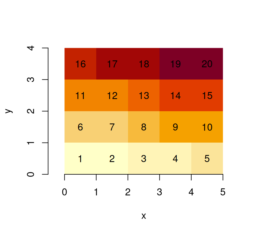

we see that $(0,0)$ is the origin of the grid (grid corner), and $1$ the coordinate value increase from one index (row, col) to the next. It means that consecutive matrix columns represent grid lines, going from south to north. Grids defined this way are regular: grid cell size is constant everywhere.

Many actual grid datasets have y coordinates (grid rows) going from North to South (top to bottom); this is realised with a negative value for delta. We see that the grid origin $(0,0)$ did not change:

attr(s, "dimensions")[[2]]$delta = -1
image(s, text_values = TRUE, axes = TRUE)

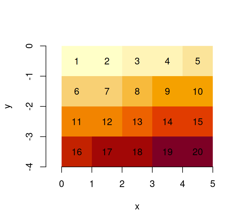
An example is the GeoTIFF carried in the package, which, as probably all data sources read through GDAL, has a negative delta for the y-coordinate:

tif = system.file("tif/L7_ETMs.tif", package = "stars")
st_dimensions(read_stars(tif))["y"]
##   from  to  offset delta                     refsys point
## y    1 352 9120761 -28.5 SIRGAS 2000 / UTM zone 25S FALSE

Raster attributes, rotated and sheared grids

Dimension tables of stars objects carry a raster attribute:

str(attr(st_dimensions(s), "raster"))
## List of 4
##  $ affine     : num [1:2] 0 0
##  $ dimensions : chr [1:2] "x" "y"
##  $ curvilinear: logi FALSE
##  $ blocksizes : NULL
##  - attr(*, "class")= chr "stars_raster"

which is a list that holds

dimensions: character, the names of raster dimensions (if any), as opposed to e.g. spectral, temporal or other dimensions
affine: numeric, the affine parameters
curvilinear: a logical indicating whether the raster is curvilinear

These fields are needed at this level, because they describe properties of the array at a higher level than individual dimensions do: a pair of dimensions forms a raster, both affine and curvilinear describe how x and y as a pair are derived from grid indexes (see below) when this cannot be done on a per-dimension basis.

With two affine parameters $a_1$ and $a_2$ , $x$ and $y$ coordinates are derived from (1-based) grid indexes $i$ and $j$ , grid offset values $o_x$ and $o_y$ , and grid cell sizes $d_x$ and $d_y$ by

$x = o_x + (i-1) d_x + (j-1) a_1$

$y = o_y + (i-1) a_2 + (j-1) d_y$ Clearly, when $a_1=a_2=0$ , $x$ and $y$ are entirely derived from their respective index, offset and cellsize.

Note that for integer indexes, the coordinates are that of the starting edge of a grid cell; to get the grid cell center of the top left grid cell (in case of a negative $d_y$ ), use $i=1.5$ and $j=1.5$ .

We can rotate grids by setting $a_1$ and $a_2$ to a non-zero value:

attr(attr(s, "dimensions"), "raster")$affine = c(0.1, 0.1)
plot(st_as_sf(s, as_points = FALSE), axes = TRUE, nbreaks = 20)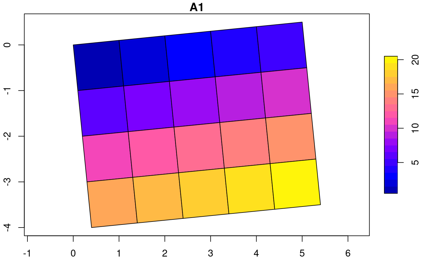

The rotation angle, in degrees, is

atan2(0.1, 1) * 180 / pi
## [1] 5.710593

Sheared grids are obtained when the two rotation coefficients, $a_1$ and $a_2$ , are unequal:

attr(attr(s, "dimensions"), "raster")$affine = c(0.1, 0.2)
plot(st_as_sf(s, as_points = FALSE), axes = TRUE, nbreaks = 20)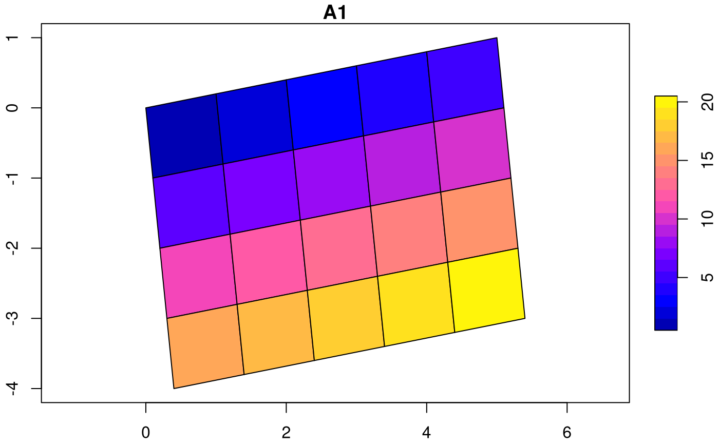

Now, the y-axis and x-axis have different rotation in degrees of respectively

atan2(c(0.1, 0.2), 1) * 180 / pi
## [1]  5.710593 11.309932

Rectilinear grids

Rectilinear grids have orthogonal axes, but do not have congruent (equally sized and shaped) cells: each axis has its own irregular subdivision.

We can define a rectilinear grid by specifying the cell boundaries, meaning for every dimension we specify one more value than the dimension size:

x = c(0, 0.5, 1, 2, 4, 5)  # 6 numbers: boundaries!
y = c(0.3, 0.5, 1, 2, 2.2) # 5 numbers: boundaries!
(r = st_as_stars(list(m = m), dimensions = st_dimensions(x = x, y = y)))
## stars object with 2 dimensions and 1 attribute
## attribute(s):
##    Min. 1st Qu. Median Mean 3rd Qu. Max.
## m     1    5.75   10.5 10.5   15.25   20
## dimension(s):
##   from to point                values x/y
## x    1  5 FALSE     [0,0.5),...,[4,5) [x]
## y    1  4 FALSE [0.3,0.5),...,[2,2.2) [y]
st_bbox(r)
## xmin ymin xmax ymax 
##  0.0  0.3  5.0  2.2
image(r, axes = TRUE, col = grey((1:20)/20))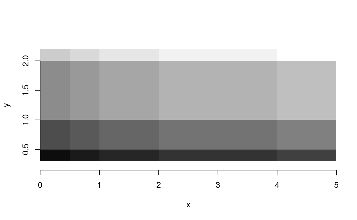

Would we leave out the last value, than stars may come up with a different cell boundary for the last cell, as this is now derived from the width of the one-but-last cell:

x = c(0, 0.5, 1, 2, 4)  # 5 numbers: offsets only!
y = c(0.3, 0.5, 1, 2)   # 4 numbers: offsets only!
(r = st_as_stars(list(m = m), dimensions = st_dimensions(x = x, y = y)))
## stars object with 2 dimensions and 1 attribute
## attribute(s):
##    Min. 1st Qu. Median Mean 3rd Qu. Max.
## m     1    5.75   10.5 10.5   15.25   20
## dimension(s):
##   from to point              values x/y
## x    1  5 FALSE   [0,0.5),...,[4,6) [x]
## y    1  4 FALSE [0.3,0.5),...,[2,3) [y]
st_bbox(r)
## xmin ymin xmax ymax 
##  0.0  0.3  6.0  3.0

This is not problematic if cells have a constant width, in which case the boundaries are reduced to an offset and delta value, irrespective whether an upper boundary is given:

x = c(0, 1, 2, 3, 4)  # 5 numbers: offsets only!
y = c(0.5, 1, 1.5, 2)   # 4 numbers: offsets only!
(r = st_as_stars(list(m = m), dimensions = st_dimensions(x = x, y = y)))
## stars object with 2 dimensions and 1 attribute
## attribute(s):
##    Min. 1st Qu. Median Mean 3rd Qu. Max.
## m     1    5.75   10.5 10.5   15.25   20
## dimension(s):
##   from to offset delta point x/y
## x    1  5      0     1 FALSE [x]
## y    1  4    0.5   0.5 FALSE [y]
st_bbox(r)
## xmin ymin xmax ymax 
##  0.0  0.5  5.0  2.5

Alternatively, one can also set the cell midpoints by specifying arguments cell_midpoints to the st_dimensions call:

x = st_as_stars(matrix(1:9, 3, 3), 
                st_dimensions(x = c(1, 2, 3), y = c(2, 3, 10), cell_midpoints = TRUE))

When the dimension is regular, this results in offset being shifted back with half a delta, or else in intervals derived from the distances between cell centers. This should obviously not be done when cell boundaries are specified.

Curvilinear grids

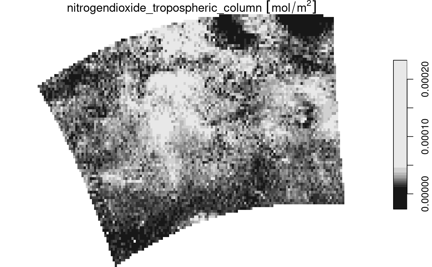
Curvilinear grids are grids whose grid lines are not straight. Rather than describing the curvature parametrically, the typical (HDF5 or NetCDF) files in which they are found have two raster layers with the longitudes and latitudes for every corresponding pixel of remaining layers.

As an example, we will use a Sentinel 5P dataset available from package starsdata; this package can be installed with

install.packages("starsdata", repos = "http://pebesma.staff.ifgi.de", type = "source")

The dataset is found here:

(s5p = system.file("sentinel5p/S5P_NRTI_L2__NO2____20180717T120113_20180717T120613_03932_01_010002_20180717T125231.nc", package = "starsdata"))
## [1] "/home/runner/work/_temp/Library/starsdata/sentinel5p/S5P_NRTI_L2__NO2____20180717T120113_20180717T120613_03932_01_010002_20180717T125231.nc"

We can construct the curvilinear stars raster by calling read_stars on the right sub-array:

subs = gdal_subdatasets(s5p)
subs[[6]]
## [1] "NETCDF:\"/home/runner/work/_temp/Library/starsdata/sentinel5p/S5P_NRTI_L2__NO2____20180717T120113_20180717T120613_03932_01_010002_20180717T125231.nc\":/PRODUCT/nitrogendioxide_tropospheric_column"

For this array, we can see the GDAL metadata under item GEOLOCATION:

gdal_metadata(subs[[6]], "GEOLOCATION")
## $LINE_OFFSET
## [1] "0"
## 
## $LINE_STEP
## [1] "1"
## 
## $PIXEL_OFFSET
## [1] "0"
## 
## $PIXEL_STEP
## [1] "1"
## 
## $SRS
## [1] "GEOGCS[\"WGS 84\",DATUM[\"WGS_1984\",SPHEROID[\"WGS 84\",6378137,298.257223563,AUTHORITY[\"EPSG\",\"7030\"]],AUTHORITY[\"EPSG\",\"6326\"]],PRIMEM[\"Greenwich\",0,AUTHORITY[\"EPSG\",\"8901\"]],UNIT[\"degree\",0.0174532925199433,AUTHORITY[\"EPSG\",\"9122\"]],AXIS[\"Latitude\",NORTH],AXIS[\"Longitude\",EAST],AUTHORITY[\"EPSG\",\"4326\"]]"
## 
## $X_BAND
## [1] "1"
## 
## $X_DATASET
## [1] "NETCDF:\"/home/runner/work/_temp/Library/starsdata/sentinel5p/S5P_NRTI_L2__NO2____20180717T120113_20180717T120613_03932_01_010002_20180717T125231.nc\":/PRODUCT/longitude"
## 
## $Y_BAND
## [1] "1"
## 
## $Y_DATASET
## [1] "NETCDF:\"/home/runner/work/_temp/Library/starsdata/sentinel5p/S5P_NRTI_L2__NO2____20180717T120113_20180717T120613_03932_01_010002_20180717T125231.nc\":/PRODUCT/latitude"
## 
## attr(,"class")
## [1] "gdal_metadata"

which reveals where, in this dataset, the longitude and latitude arrays are kept.

nit.c = read_stars(subs[[6]]) 
## Warning in CPL_read_gdal(as.character(x), as.character(options),
## as.character(driver), : GDAL Message 1: The dataset has several variables that
## could be identified as vector fields, but not all share the same primary
## dimension. Consequently they will be ignored.
## Warning in CPL_read_gdal(as.character(x), as.character(options),
## as.character(driver), : GDAL Message 1: The dataset has several variables that
## could be identified as vector fields, but not all share the same primary
## dimension. Consequently they will be ignored.
## Warning in CPL_read_gdal(as.character(x), as.character(options),
## as.character(driver), : GDAL Message 1: The dataset has several variables that
## could be identified as vector fields, but not all share the same primary
## dimension. Consequently they will be ignored.
## Warning in CPL_read_gdal(as.character(x), as.character(options),
## as.character(driver), : GDAL Message 1: The dataset has several variables that
## could be identified as vector fields, but not all share the same primary
## dimension. Consequently they will be ignored.
## Warning in CPL_read_gdal(as.character(x), as.character(options),
## as.character(driver), : GDAL Message 1: The dataset has several variables that
## could be identified as vector fields, but not all share the same primary
## dimension. Consequently they will be ignored.
## Warning in CPL_read_gdal(as.character(x), as.character(options),
## as.character(driver), : GDAL Message 1: The dataset has several variables that
## could be identified as vector fields, but not all share the same primary
## dimension. Consequently they will be ignored.
## Warning in CPL_read_gdal(as.character(x), as.character(options),
## as.character(driver), : GDAL Message 1: The dataset has several variables that
## could be identified as vector fields, but not all share the same primary
## dimension. Consequently they will be ignored.
## Warning in CPL_read_gdal(as.character(x), as.character(options),
## as.character(driver), : GDAL Message 1: The dataset has several variables that
## could be identified as vector fields, but not all share the same primary
## dimension. Consequently they will be ignored.
## Warning in CPL_read_gdal(as.character(x), as.character(options),
## as.character(driver), : GDAL Message 1: The dataset has several variables that
## could be identified as vector fields, but not all share the same primary
## dimension. Consequently they will be ignored.
## Warning in CPL_read_gdal(as.character(x), as.character(options),
## as.character(driver), : GDAL Message 1: The dataset has several variables that
## could be identified as vector fields, but not all share the same primary
## dimension. Consequently they will be ignored.
threshold = units::set_units(9e+36, mol/m^2)
nit.c[[1]][nit.c[[1]] > threshold] = NA
nit.c
## stars object with 3 dimensions and 1 attribute
## attribute(s):
##                                                   Min.      1st Qu.
## nitrogendioxide_tropospheri... [mol/m^2] -3.301083e-05 1.868205e-05
##                                                Median         Mean      3rd Qu.
## nitrogendioxide_tropospheri... [mol/m^2] 2.622178e-05 2.898976e-05 3.629641e-05
##                                                  Max. NA's
## nitrogendioxide_tropospheri... [mol/m^2] 0.0003924858  330
## dimension(s):
##      from  to         offset  refsys                             values x/y
## x       1 450             NA  WGS 84 [450x278] -5.811 [°],...,30.95 [°] [x]
## y       1 278             NA  WGS 84  [450x278] 28.36 [°],...,51.47 [°] [y]
## time    1   1 2018-07-17 UTC POSIXct                               NULL    
## curvilinear grid

The curvilinear array has the actual arrays (raster layers, matrices) with longitude and latitude values read in its dimension table. We can plot this file:

plot(nit.c, breaks = "equal", reset = FALSE, axes = TRUE, as_points = TRUE, 
         pch = 16,  logz = TRUE, key.length = 1)
## Warning in NextMethod(): NaNs produced
## Warning in plot.sf(x, pal = col, ...): NaNs produced
maps::map('world', add = TRUE, col = 'red')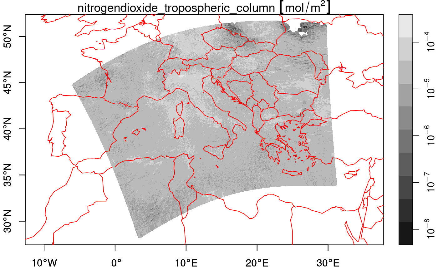

plot(nit.c, breaks = "equal", reset = FALSE, axes = TRUE, as_points = FALSE, 
         border = NA, logz = TRUE, key.length = 1)
## Warning in NextMethod(): NaNs produced
## Warning in plot.sf(x, pal = col, ...): NaNs produced
maps::map('world', add = TRUE, col = 'red')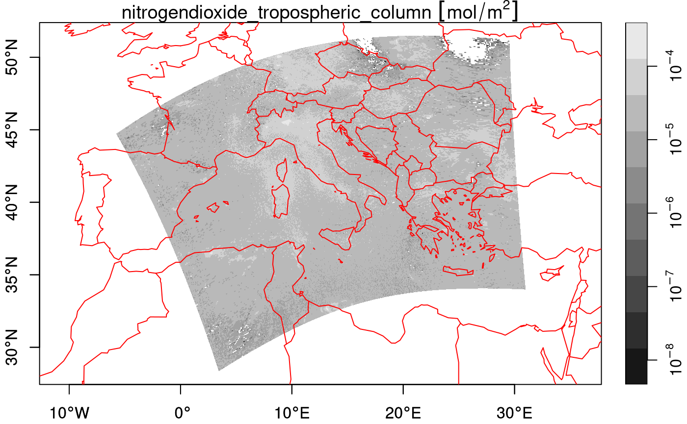

We can downsample the data by

(nit.c_ds = stars:::st_downsample(nit.c, 8))
## stars object with 3 dimensions and 1 attribute
## attribute(s):
##                                                   Min.     1st Qu.       Median
## nitrogendioxide_tropospheri... [mol/m^2] -1.847503e-05 1.85778e-05 2.700901e-05
##                                                Mean      3rd Qu.         Max.
## nitrogendioxide_tropospheri... [mol/m^2] 2.9113e-05 3.642568e-05 0.0001363282
##                                          NA's
## nitrogendioxide_tropospheri... [mol/m^2]   32
## dimension(s):
##      from to         offset  refsys                           values x/y
## x       1 50             NA  WGS 84 [50x31] -5.811 [°],...,30.14 [°] [x]
## y       1 31             NA  WGS 84  [50x31] 28.78 [°],...,51.47 [°] [y]
## time    1  1 2018-07-17 UTC POSIXct                             NULL    
## curvilinear grid
plot(nit.c_ds, breaks = "equal", reset = FALSE, axes = TRUE, as_points = TRUE, 
         pch = 16, logz = TRUE, key.length = 1)
## Warning in NextMethod(): NaNs produced
## Warning in plot.sf(x, pal = col, ...): NaNs produced
maps::map('world', add = TRUE, col = 'red')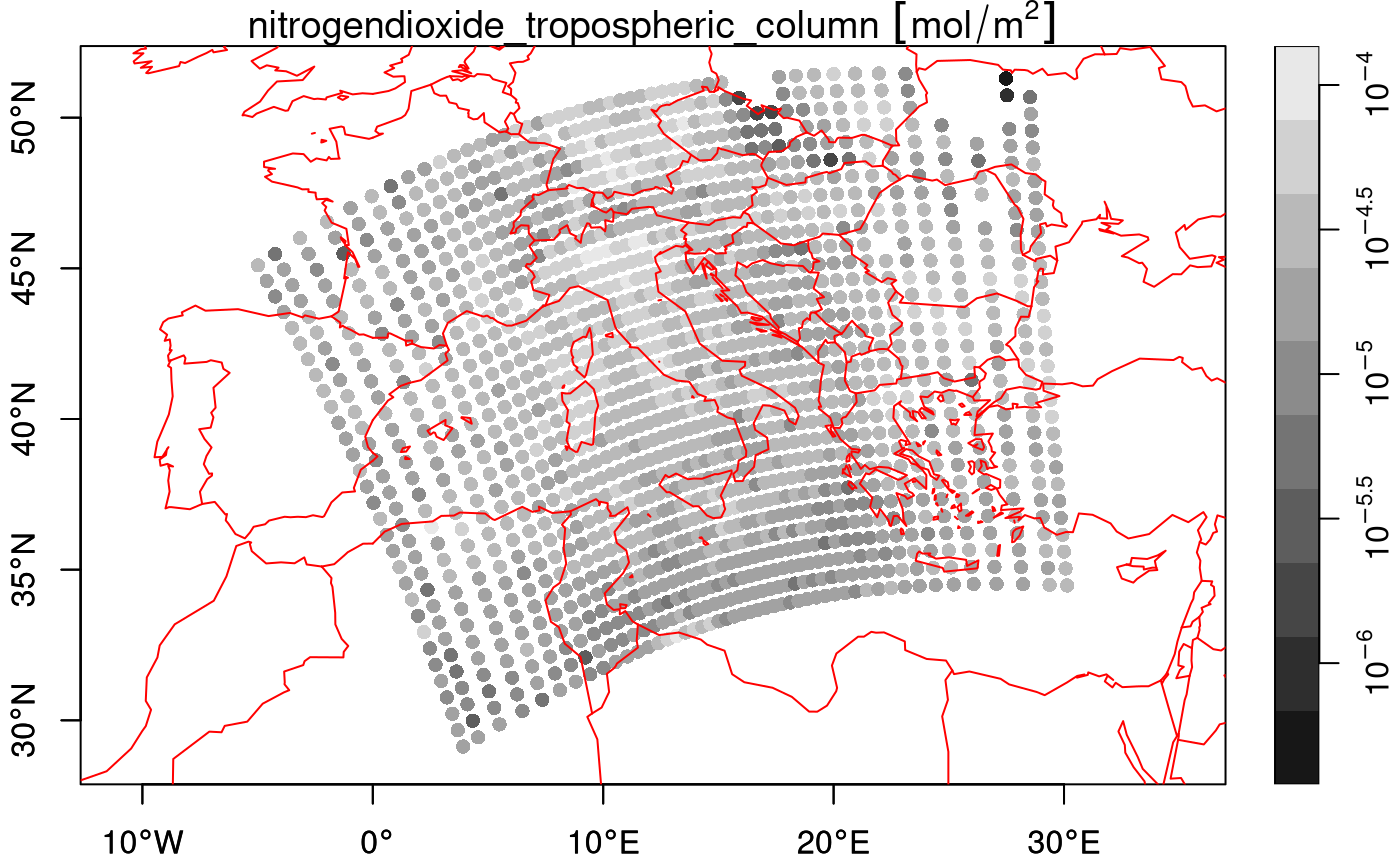

which doesn’t look nice, but plotting the cells as polygons looks better:

plot(nit.c_ds, breaks = "equal", reset = FALSE, axes = TRUE, as_points = FALSE, 
         border = NA, logz = TRUE, key.length = 1)
## Warning in NextMethod(): NaNs produced
## Warning in plot.sf(x, pal = col, ...): NaNs produced
maps::map('world', add = TRUE, col = 'red')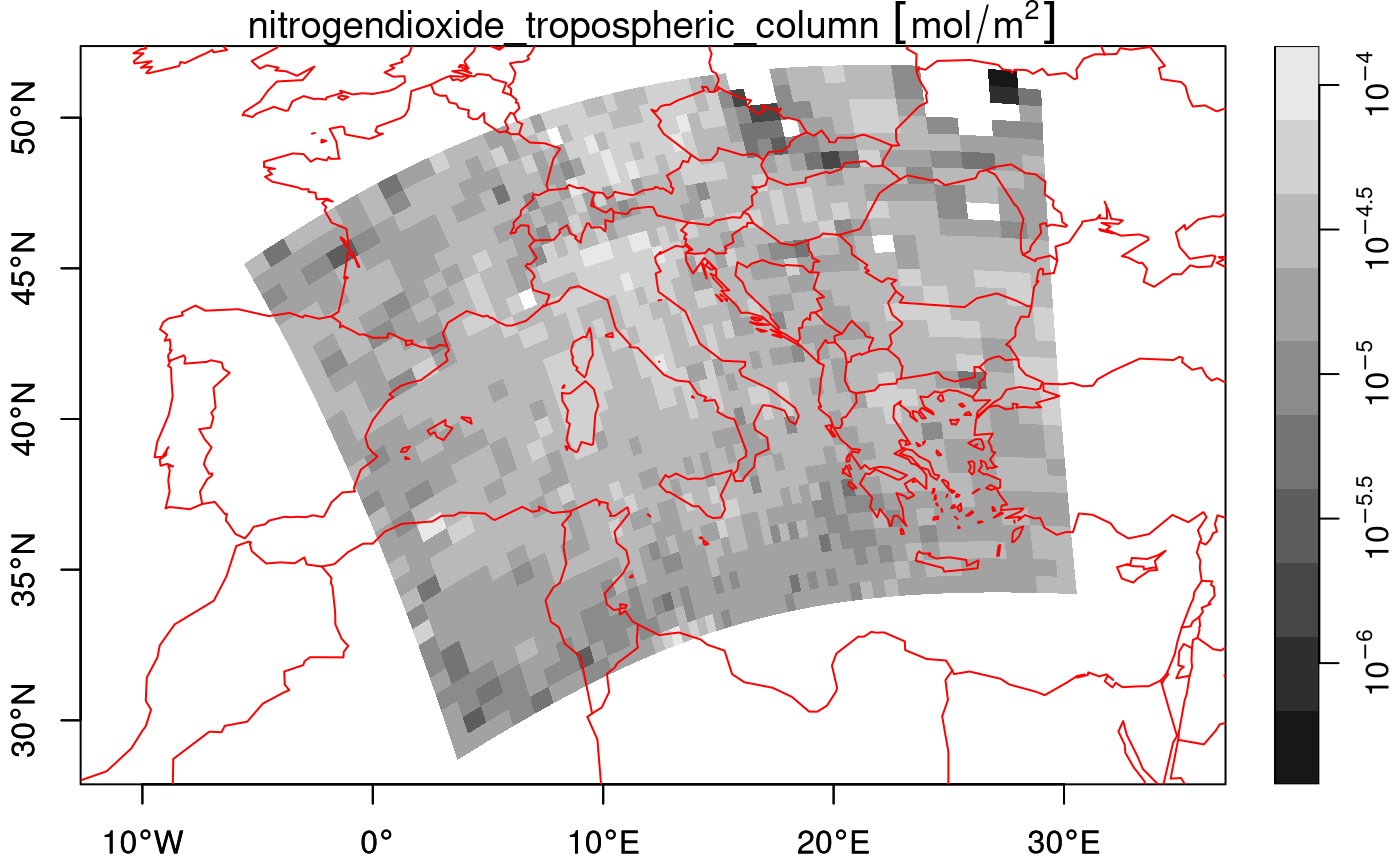

Another approach would be to warp the curvilinear grid to a regular grid, e.g. by