1. introduction

Edzer Pebesma

Package stars provides infrastructure for data cubes, array data with labeled dimensions, with emphasis on arrays where some of the dimensions relate to time and/or space.

Spatial data cubes are arrays with one or more spatial dimensions. Raster data cubes have at least two spatial dimensions that form the raster tesselation. Vector data cubes have at least one spatial dimension that may for instance reflect a polygon tesselation, or a set of point locations. Conversions between the two (rasterization, polygonization) are provided. Vector data are represented by simple feature geometries (packages sf). Tidyverse methods are provided.

The stars package is loaded by

library(stars)
## Loading required package: abind
## Loading required package: sf
## Linking to GEOS 3.10.2, GDAL 3.4.1, PROJ 8.2.1; sf_use_s2() is TRUE

Spatiotemporal arrays are stored in objects of class stars; methods for class stars currently available are

methods(class = "stars")
##  [1] [                 [[<-              [<-               %in%             
##  [5] $<-               adrop             aggregate         aperm            
##  [9] as.data.frame     as.POSIXct        c                 coerce           
## [13] contour           cut               dim               dimnames         
## [17] dimnames<-        droplevels        expand_dimensions hist             
## [21] image             initialize        is.na             Math             
## [25] merge             Ops               plot              prcomp           
## [29] predict           print             show              slotsFromS3      
## [33] split             st_apply          st_area           st_as_sf         
## [37] st_as_sfc         st_as_stars       st_bbox           st_coordinates   
## [41] st_crop           st_crs            st_crs<-          st_dimensions    
## [45] st_dimensions<-   st_downsample     st_extract        st_geometry      
## [49] st_geotransform   st_geotransform<- st_interpolate_aw st_intersects    
## [53] st_join           st_mosaic         st_normalize      st_redimension   
## [57] st_rotate         st_sample         st_set_bbox       st_transform     
## [61] st_write          time              write_stars      
## see '?methods' for accessing help and source code

(tidyverse methods are only visible after loading package tidyverse).

Reading a satellite image

We can read a satellite image through GDAL, e.g. from a GeoTIFF file in the package:

tif = system.file("tif/L7_ETMs.tif", package = "stars")
x = read_stars(tif)
plot(x, axes = TRUE)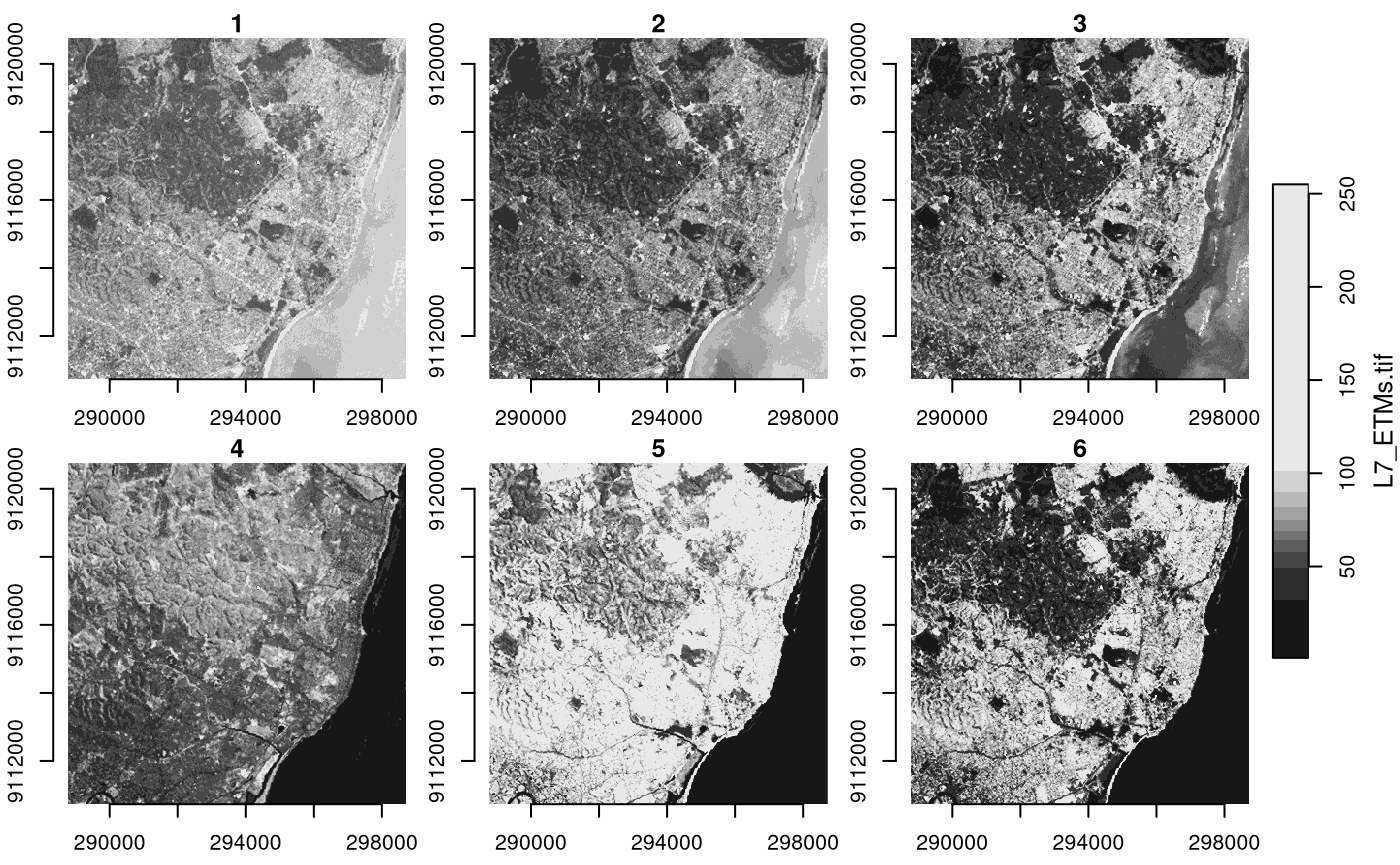

We see that the image is geographically referenced (has coordinate values along axes), and that the object returned (x) has three dimensions called x, y and band, and has one attribute:

x
## stars object with 3 dimensions and 1 attribute
## attribute(s):
##              Min. 1st Qu. Median     Mean 3rd Qu. Max.
## L7_ETMs.tif     1      54     69 68.91242      86  255
## dimension(s):
##      from  to  offset delta                     refsys point x/y
## x       1 349  288776  28.5 SIRGAS 2000 / UTM zone 25S FALSE [x]
## y       1 352 9120761 -28.5 SIRGAS 2000 / UTM zone 25S FALSE [y]
## band    1   6      NA    NA                         NA    NA

Each dimension has a name; the meaning of the fields of a single dimension are:

field	meaning
from	the origin index (1)
to	the final index (dim(x)[i])
offset	the start value for this dimension (pixel boundary), if regular
delta	the step (pixel, cell) size for this dimension, if regular
refsys	the reference system, or proj4string
point	logical; whether cells refer to points, or intervals
values	the sequence of values for this dimension (e.g., geometries), if irregular

This means that for an index i (starting at $i=1$) along a certain dimension, the corresponding dimension value (coordinate, time) is $\mbox{offset} + (i-1) \times \mbox{delta}$. This value then refers to the start (edge) of the cell or interval; in order to get the interval middle or cell centre, one needs to add half an offset.

Dimension band is a simple sequence from 1 to 6. Since bands refer to colors, one could put their wavelength values in the values field.

For this particular dataset (and most other raster datasets), we see that delta for dimension y is negative: this means that consecutive array values have decreasing $y$ values: cell indexes increase from top to bottom, in the direction opposite to the $y$ axis.

read_stars reads all bands from a raster dataset, or optionally a subset of raster datasets, into a single stars array structure. While doing so, raster values (often UINT8 or UINT16) are converted to double (numeric) values, and scaled back to their original values if needed if the file encodes the scaling parameters.

The data structure stars is a generalization of the tbl_cube found in cubelyr; we can convert to that by

library(cubelyr)
as.tbl_cube(x)
## Source: local array [737,088 x 3]
## D: x [dbl, 349]
## D: y [dbl, 352]
## D: band [int, 6]
## M: L7_ETMs.tif [dbl[,352,6]]

but this will cause a loss of certain properties (cell size, reference system, vector geometries)

Switching attributes to dimensions and back

(x.spl = split(x, "band"))
## stars object with 2 dimensions and 6 attributes
## attribute(s):
##     Min. 1st Qu. Median     Mean 3rd Qu. Max.
## X1    47      67     78 79.14772      89  255
## X2    32      55     66 67.57465      79  255
## X3    21      49     63 64.35886      77  255
## X4     9      52     63 59.23541      75  255
## X5     1      63     89 83.18266     112  255
## X6     1      32     60 59.97521      88  255
## dimension(s):
##   from  to  offset delta                     refsys point x/y
## x    1 349  288776  28.5 SIRGAS 2000 / UTM zone 25S FALSE [x]
## y    1 352 9120761 -28.5 SIRGAS 2000 / UTM zone 25S FALSE [y]
merge(x.spl)
## stars object with 3 dimensions and 1 attribute
## attribute(s):
##                    Min. 1st Qu. Median     Mean 3rd Qu. Max.
## X1.X2.X3.X4.X5.X6     1      54     69 68.91242      86  255
## dimension(s):
##            from  to  offset delta                     refsys point    values
## x             1 349  288776  28.5 SIRGAS 2000 / UTM zone 25S FALSE      NULL
## y             1 352 9120761 -28.5 SIRGAS 2000 / UTM zone 25S FALSE      NULL
## attributes    1   6      NA    NA                         NA    NA X1,...,X6
##            x/y
## x          [x]
## y          [y]
## attributes

We see that the newly created dimension lost its name, and the single attribute got a default name. We can set attribute names with setNames, and dimension names and values with st_set_dimensions:

merge(x.spl) |>
  setNames(names(x)) |> 
  st_set_dimensions(3, values = paste0("band", 1:6)) |>
  st_set_dimensions(names = c("x", "y", "band"))
## stars object with 3 dimensions and 1 attribute
## attribute(s):
##              Min. 1st Qu. Median     Mean 3rd Qu. Max.
## L7_ETMs.tif     1      54     69 68.91242      86  255
## dimension(s):
##      from  to  offset delta                     refsys point          values
## x       1 349  288776  28.5 SIRGAS 2000 / UTM zone 25S FALSE            NULL
## y       1 352 9120761 -28.5 SIRGAS 2000 / UTM zone 25S FALSE            NULL
## band    1   6      NA    NA                         NA    NA band1,...,band6
##      x/y
## x    [x]
## y    [y]
## band

Subsetting

Besides the tidyverse subsetting and selection operators explained in this vignette, we can also use [ and [[.

Since stars objects are a list of arrays with a metadata table describing dimensions, list extraction (and assignment) works as expected:

class(x[[1]])
## [1] "array"
dim(x[[1]])
##    x    y band 
##  349  352    6
x$two = 2 * x[[1]]
x
## stars object with 3 dimensions and 2 attributes
## attribute(s):
##              Min. 1st Qu. Median      Mean 3rd Qu. Max.
## L7_ETMs.tif     1      54     69  68.91242      86  255
## two             2     108    138 137.82484     172  510
## dimension(s):
##      from  to  offset delta                     refsys point x/y
## x       1 349  288776  28.5 SIRGAS 2000 / UTM zone 25S FALSE [x]
## y       1 352 9120761 -28.5 SIRGAS 2000 / UTM zone 25S FALSE [y]
## band    1   6      NA    NA                         NA    NA

At this level, we can work with array objects directly.

The stars subset operator [ works a bit different: its

• first argument selects attributes
• second argument selects the first dimension
• third argument selects the second dimension, etc

Thus,

x["two", 1:10, , 2:4]
## stars object with 3 dimensions and 1 attribute
## attribute(s):
##      Min. 1st Qu. Median     Mean 3rd Qu. Max.
## two    36     100    116 119.7326     136  470
## dimension(s):
##      from  to  offset delta                     refsys point x/y
## x       1  10  288776  28.5 SIRGAS 2000 / UTM zone 25S FALSE [x]
## y       1 352 9120761 -28.5 SIRGAS 2000 / UTM zone 25S FALSE [y]
## band    2   4      NA    NA                         NA    NA

selects the second attribute, the first 10 columns (x-coordinate), all rows, and bands 2-4.

Alternatively, when [ is given a single argument of class sf, sfc or bbox, [ will work as a crop operator:

circle = st_sfc(st_buffer(st_point(c(293749.5, 9115745)), 400), crs = st_crs(x))
plot(x[circle][, , , 1], reset = FALSE)
plot(circle, col = NA, border = 'red', add = TRUE, lwd = 2)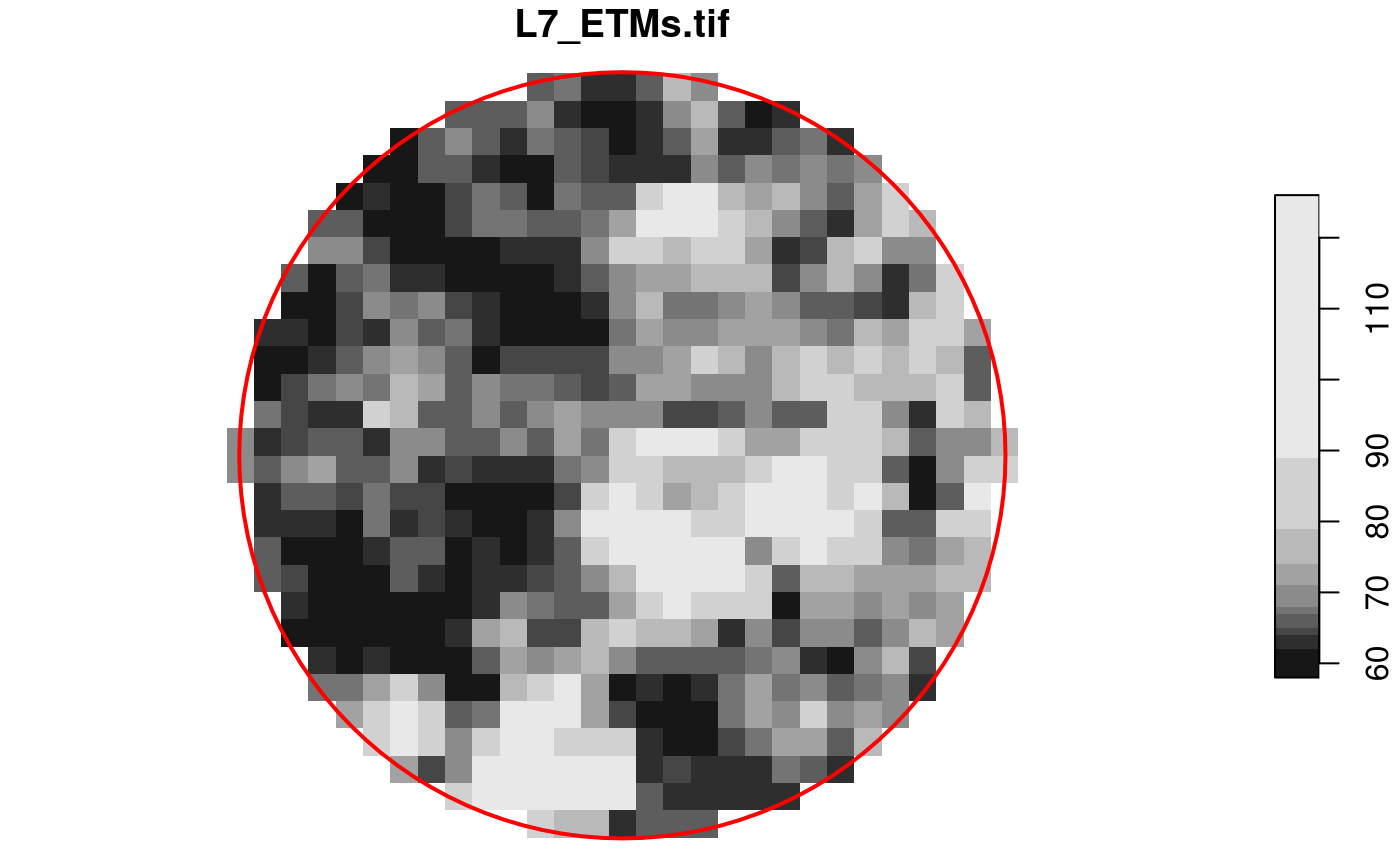

Overviews

We can read rasters at a lower resolution when they contain so-called overviews. For this GeoTIFF file, they were created with the gdaladdo utility, in particular

gdaladdo -r average L7_ETMs.tif  2 4 8 16

which adds coarse resolution versions by using the average resampling method to compute values based on blocks of pixels. These can be read by

x1 = read_stars(tif, options = c("OVERVIEW_LEVEL=1"))
x2 = read_stars(tif, options = c("OVERVIEW_LEVEL=2"))
x3 = read_stars(tif, options = c("OVERVIEW_LEVEL=3"))
dim(x1)
##    x    y band 
##   88   88    6
dim(x2)
##    x    y band 
##   44   44    6
dim(x3)
##    x    y band 
##   22   22    6
par(mfrow = c(1, 3), mar = rep(0.2, 4))
image(x1[,,,1])
image(x2[,,,1])
image(x3[,,,1])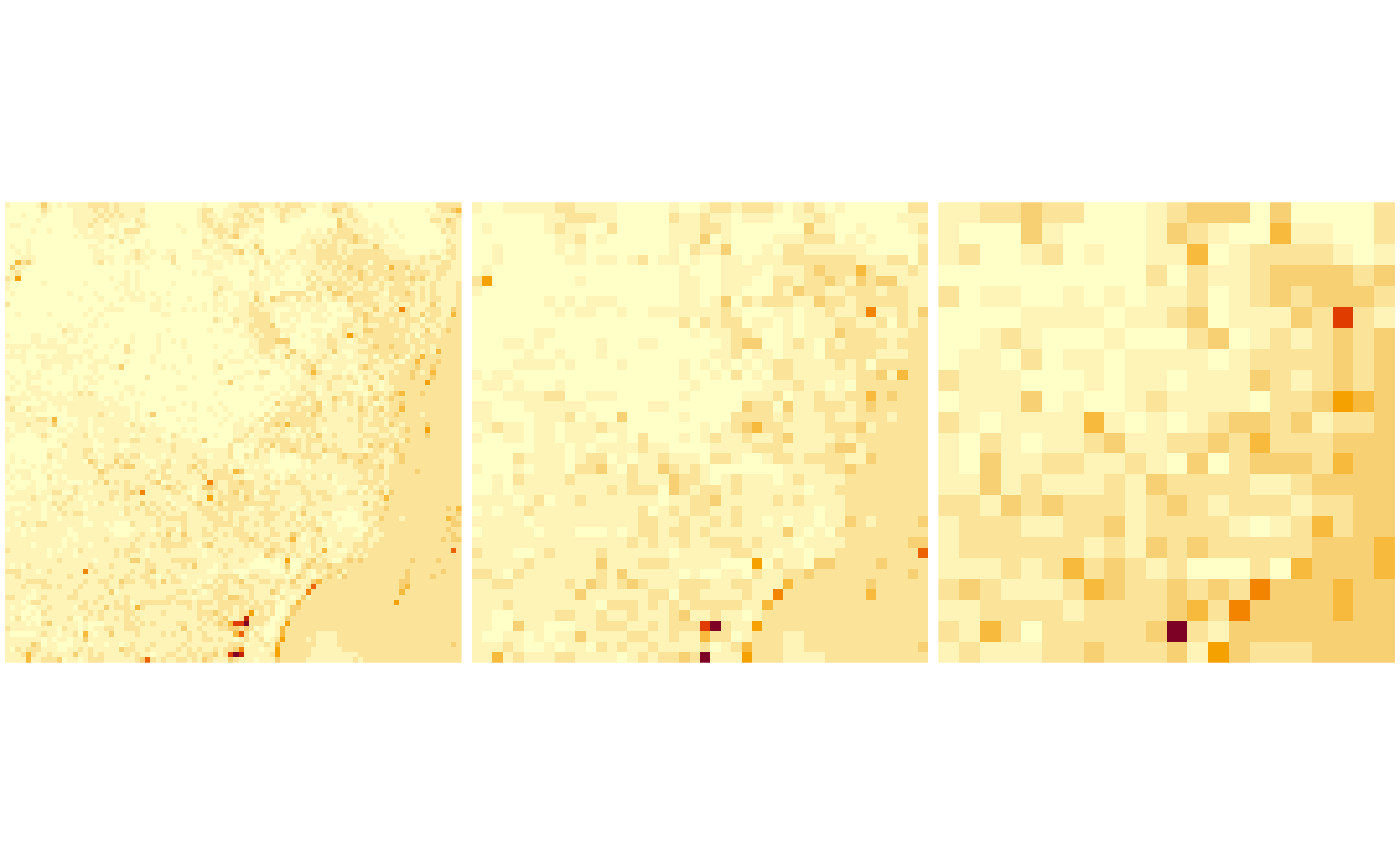

Reading a raster time series: NetCDF

Another example is when we read raster time series model outputs in a NetCDF file, e.g. by

system.file("nc/bcsd_obs_1999.nc", package = "stars") |>
    read_stars() -> w
## pr, tas,

We see that

w
## stars object with 3 dimensions and 2 attributes
## attribute(s):
##                 Min.   1st Qu.   Median      Mean   3rd Qu.      Max. NA's
## pr [mm/m]  0.5900000 56.139999 81.88000 101.26433 121.07250 848.54999 7116
## tas [C]   -0.4209678  8.898887 15.65763  15.48932  21.77979  29.38581 7116
## dimension(s):
##      from to offset  delta  refsys                    values x/y
## x       1 81    -85  0.125      NA                      NULL [x]
## y       1 33  37.12 -0.125      NA                      NULL [y]
## time    1 12     NA     NA POSIXct 1999-01-31,...,1999-12-31

For this dataset we can see that

• variables have units associated (and a wrong unit, C is assigned to temperature)
• time is now a dimension, with proper units and time steps

Alternatively, this dataset can be read using read_ncdf, as in

system.file("nc/bcsd_obs_1999.nc", package = "stars") |>
    read_ncdf()
## no 'var' specified, using pr, tas
## other available variables:
##  latitude, longitude, time
## Will return stars object with 32076 cells.
## No projection information found in nc file. 
##  Coordinate variable units found to be degrees, 
##  assuming WGS84 Lat/Lon.
## stars object with 3 dimensions and 2 attributes
## attribute(s):
##                 Min.   1st Qu.   Median      Mean   3rd Qu.      Max. NA's
## pr [mm/m]  0.5900000 56.139999 81.88000 101.26433 121.07250 848.54999 7116
## tas [C]   -0.4209678  8.898887 15.65763  15.48932  21.77979  29.38581 7116
## dimension(s):
##           from to offset delta  refsys                    values x/y
## longitude    1 81    -85 0.125  WGS 84                      NULL [x]
## latitude     1 33     33 0.125  WGS 84                      NULL [y]
## time         1 12     NA    NA POSIXct 1999-01-31,...,1999-12-31

The difference between read_ncdf and read_stars for NetCDF files is that the former uses package RNetCDF to directly read the NetCDF file, where the latter uses the GDAL driver for NetCDF files.

Reading datasets from multiple files

Model data are often spread across many files. An example of a 0.25 degree grid, global daily sea surface temperature product is found here; the subset from 1981 used below was downloaded from a NOAA ftp site that is no longer available in this form. (ftp site used to be eclipse.ncdc.noaa.gov/pub/OI-daily-v2/NetCDF/1981/AVHRR/).

We read the data by giving read_stars a vector with character names:

x = c(
"avhrr-only-v2.19810901.nc",
"avhrr-only-v2.19810902.nc",
"avhrr-only-v2.19810903.nc",
"avhrr-only-v2.19810904.nc",
"avhrr-only-v2.19810905.nc",
"avhrr-only-v2.19810906.nc",
"avhrr-only-v2.19810907.nc",
"avhrr-only-v2.19810908.nc",
"avhrr-only-v2.19810909.nc"
)
# see the second vignette:
# install.packages("starsdata", repos = "http://pebesma.staff.ifgi.de", type = "source")
file_list = system.file(paste0("netcdf/", x), package = "starsdata")
(y = read_stars(file_list, quiet = TRUE))
## stars object with 4 dimensions and 4 attributes
## attribute(s), summary of first 1e+05 cells:
##                Min. 1st Qu. Median       Mean 3rd Qu. Max.  NA's
## sst [°*C]     -1.80   -1.19  -1.05 -0.3201670   -0.20 9.36 13360
## anom [°*C]    -4.69   -0.06   0.52  0.2299385    0.71 3.70 13360
## err [°*C]      0.11    0.30   0.30  0.2949421    0.30 0.48 13360
## ice [percent]  0.01    0.73   0.83  0.7657695    0.87 1.00 27377
## dimension(s):
##      from   to         offset  delta  refsys x/y
## x       1 1440              0   0.25      NA [x]
## y       1  720             90  -0.25      NA [y]
## zlev    1    1          0 [m]     NA      NA    
## time    1    9 1981-09-01 UTC 1 days POSIXct

Next, we select sea surface temperature (sst), and drop the singular zlev (depth) dimension using adrop:

library(dplyr)
## 
## Attaching package: 'dplyr'
## The following objects are masked from 'package:stats':
## 
##     filter, lag
## The following objects are masked from 'package:base':
## 
##     intersect, setdiff, setequal, union
library(abind)
z <- y |> select(sst) |> adrop()

We can now graph the sea surface temperature (SST) using ggplot, which needs data in a long table form, and without units:

# convert POSIXct time to character, to please ggplot's facet_wrap()
z1 = st_set_dimensions(z, 3, values = as.character(st_get_dimension_values(z, 3)))
library(ggplot2)
library(viridis)
## Loading required package: viridisLite
library(ggthemes)
ggplot() +  
  geom_stars(data = z1[1], alpha = 0.8, downsample = c(10, 10, 1)) + 
  facet_wrap("time") +
  scale_fill_viridis() +
  coord_equal() +
  theme_map() +
  theme(legend.position = "bottom") +
  theme(legend.key.width = unit(2, "cm"))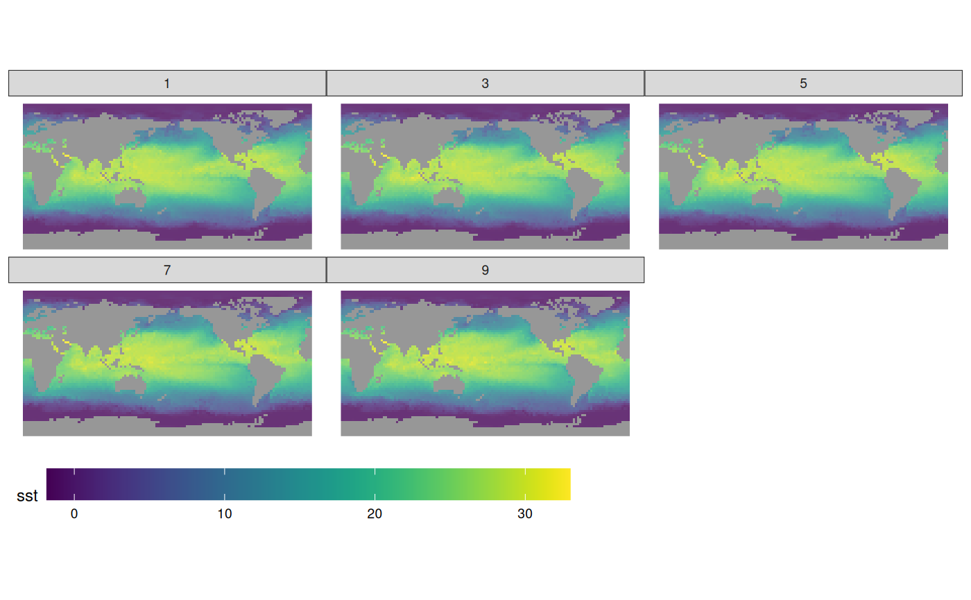

Writing stars objects to disk

We can write a stars object to disk by using write_stars; this used the GDAL write engine. Writing NetCDF files without going through the GDAL interface is currently not supported. write_stars currently writes only a single attribute:

write_stars(adrop(y[1]), "sst.tif")

See the explanation of merge above to see how multiple attributes can be merged (folded) into a dimension.

Cropping a raster’s extent

Using a curvilinear grid, taken from the example of read_ncdf:

prec_file = system.file("nc/test_stageiv_xyt.nc", package = "stars")
prec = read_ncdf(prec_file, curvilinear = c("lon", "lat"))
## no 'var' specified, using Total_precipitation_surface_1_Hour_Accumulation
## other available variables:
##  lat, lon, time
## Will return stars object with 236118 cells.
## No projection information found in nc file. 
##  Coordinate variable units found to be degrees, 
##  assuming WGS84 Lat/Lon.
##plot(prec) ## gives error about unique breaks
## remove NAs, zeros, and give a large number
## of breaks (used for validating in detail)
qu_0_omit = function(x, ..., n = 22) {
  if (inherits(x, "units"))
    x = units::drop_units(na.omit(x))
  c(0, quantile(x[x > 0], seq(0, 1, length.out = n)))
}
library(dplyr) # loads slice generic
prec_slice = slice(prec, index = 17, along = "time")
plot(prec_slice, border = NA, breaks = qu_0_omit(prec_slice[[1]]), reset = FALSE)
nc = sf::read_sf(system.file("gpkg/nc.gpkg", package = "sf"), "nc.gpkg")
plot(st_geometry(nc), add = TRUE, reset = FALSE, col = NA, border = 'red')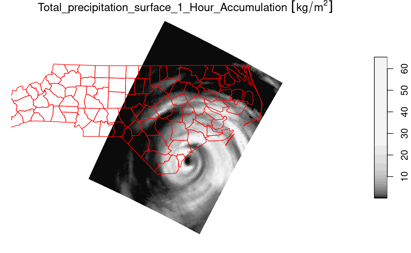

We can now crop the grid to those cells falling in

nc = st_transform(nc, st_crs(prec_slice)) # datum transformation
plot(prec_slice[nc], border = NA, breaks = qu_0_omit(prec_slice[[1]]), reset = FALSE)
plot(st_geometry(nc), add = TRUE, reset = FALSE, col = NA, border = 'red')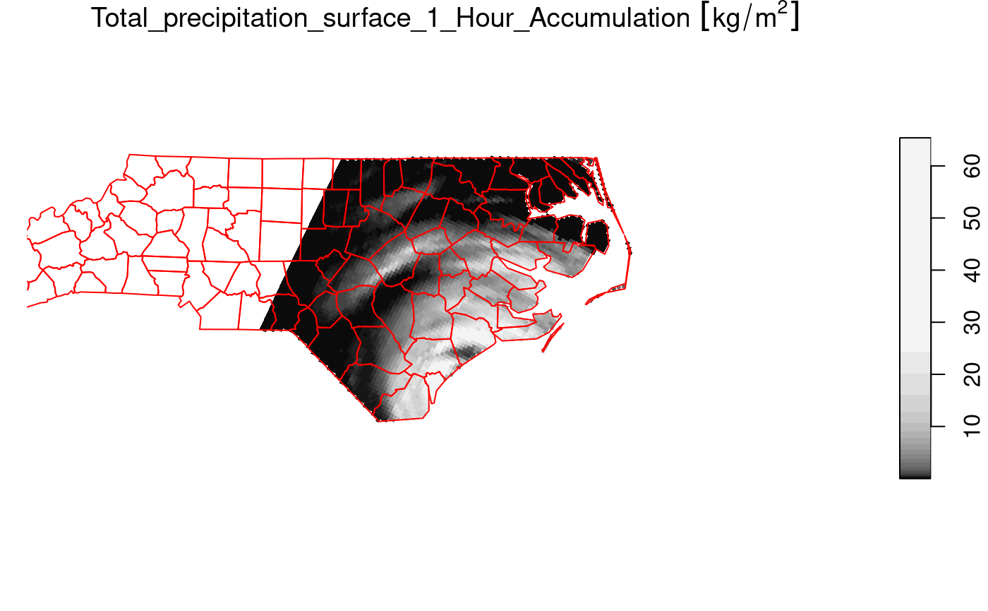

The selection prec_slice[nc] essentially calls st_crop(prec_slice, nc) to get a cropped selection. What happened here is that all cells not intersecting with North Carolina (sea) are set to NA values. For regular grids, the extent of the resulting stars object is also be reduced (cropped) by default; this can be controlled with the crop parameter to st_crop and [.stars.

Vector data cube example

Like tbl_cube, stars arrays have no limits to the number of dimensions they handle. An example is the origin-destination (OD) matrix, by time and travel mode.

OD: space x space x travel mode x time x time

We create a 5-dimensional matrix of traffic between regions, by day, by time of day, and by travel mode. Having day and time of day each as dimension is an advantage when we want to compute patterns over the day, for a certain period.

nc = st_read(system.file("gpkg/nc.gpkg", package="sf")) 
## Reading layer `nc.gpkg' from data source 
##   `/home/runner/work/_temp/Library/sf/gpkg/nc.gpkg' using driver `GPKG'
## Simple feature collection with 100 features and 14 fields
## Geometry type: MULTIPOLYGON
## Dimension:     XY
## Bounding box:  xmin: -84.32385 ymin: 33.88199 xmax: -75.45698 ymax: 36.58965
## Geodetic CRS:  NAD27
to = from = st_geometry(nc) # 100 polygons: O and D regions
mode = c("car", "bike", "foot") # travel mode
day = 1:100 # arbitrary
library(units)
## udunits database from /usr/share/xml/udunits/udunits2.xml
units(day) = as_units("days since 2015-01-01")
hour = set_units(0:23, h) # hour of day
dims = st_dimensions(origin = from, destination = to, mode = mode, day = day, hour = hour)
(n = dim(dims))
##      origin destination        mode         day        hour 
##         100         100           3         100          24
traffic = array(rpois(prod(n), 10), dim = n) # simulated traffic counts
(st = st_as_stars(list(traffic = traffic),  dimensions = dims))
## stars object with 5 dimensions and 1 attribute
## attribute(s), summary of first 1e+05 cells:
##          Min. 1st Qu. Median    Mean 3rd Qu. Max.
## traffic     0       8     10 9.99961      12   26
## dimension(s):
##             from  to                      offset                       delta
## origin         1 100                          NA                          NA
## destination    1 100                          NA                          NA
## mode           1   3                          NA                          NA
## day            1 100 1 [(days since 2015-01-01)] 1 [(days since 2015-01-01)]
## hour           1  24                       0 [h]                       1 [h]
##              refsys point
## origin        NAD27 FALSE
## destination   NAD27 FALSE
## mode             NA FALSE
## day         udunits FALSE
## hour        udunits FALSE
##                                                                    values
## origin      MULTIPOLYGON (((-81.47276...,...,MULTIPOLYGON (((-78.65572...
## destination MULTIPOLYGON (((-81.47276...,...,MULTIPOLYGON (((-78.65572...
## mode                                                     car , bike, foot
## day                                                                  NULL
## hour                                                                 NULL

This array contains the simple feature geometries of origin and destination so that we can directly plot every slice without additional table joins. If we want to represent such an array as a tbl_cube, the simple feature geometry dimensions need to be replaced by indexes:

st |> as.tbl_cube()
## Source: local array [72,000,000 x 5]
## D: origin [int, 100]
## D: destination [int, 100]
## D: mode [chr, 3]
## D: day [[(days since 2015-01-01)], 100]
## D: hour [[h], 24]
## M: traffic [int[,100,3,100,24]]

The following demonstrates how we can use dplyr to filter travel mode bike, and compute mean bike traffic by hour of day:

b <- st |> 
  as.tbl_cube() |> 
  filter(mode == "bike") |> 
  group_by(hour) |>
  summarise(traffic = mean(traffic)) |> 
  as.data.frame()
require(ggforce) # for plotting a units variable
## Loading required package: ggforce
ggplot() +  
  geom_line(data = b, aes(x = hour, y = traffic))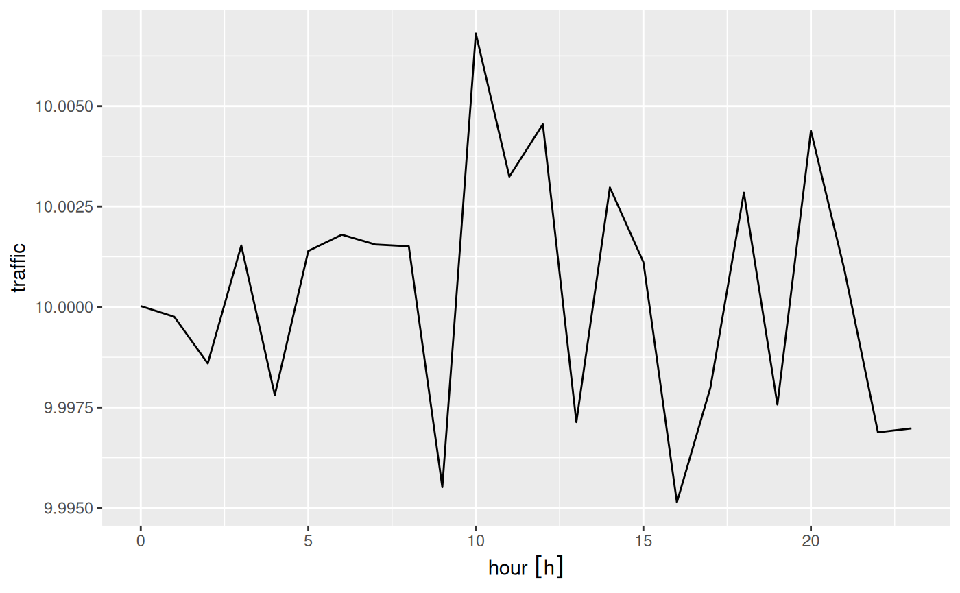
## Warning: The `scale_name` argument of `continuous_scale()` is deprecated as of ggplot2
## 3.5.0.
## This warning is displayed once every 8 hours.
## Call `lifecycle::last_lifecycle_warnings()` to see where this warning was
## generated.

Extracting at point locations, aggregating over polygons

Data cube values at point location can be extracted by st_extract, an example is found in vignette 7

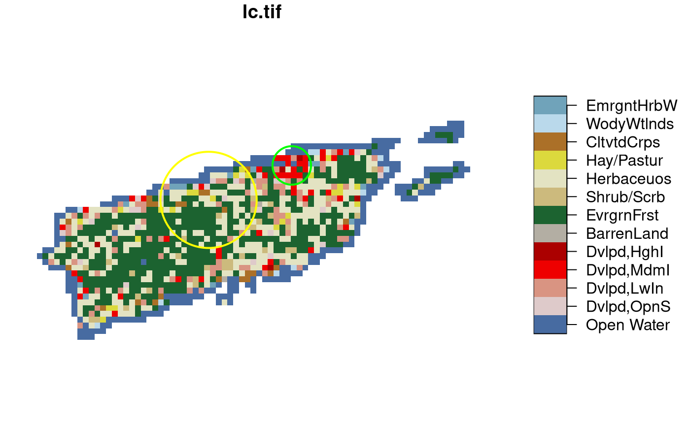
Aggregates, such as mean, maximum or modal values can be obtained by aggregate. In this example we use a categorical raster, and try to find the modal (most frequent) class within two circular polygons:

s = system.file("tif/lc.tif", package = "stars")
r = read_stars(s, proxy = FALSE) |> droplevels()
levels(r[[1]]) = abbreviate(levels(r[[1]]), 10) # shorten text labels
st_point(c(3190631, 3125)) |> st_sfc(crs = st_crs(r)) |> st_buffer(25000) -> pol1
st_point(c(3233847, 21027)) |> st_sfc(crs = st_crs(r)) |> st_buffer(10000) -> pol2
if (isTRUE(dev.capabilities()$rasterImage == "yes")) {
  plot(r, reset = FALSE, key.pos = 4)
  plot(c(pol1, pol2), col = NA, border = c('yellow', 'green'), lwd = 2, add = TRUE)
}

To find the modal value, we need a function that gives back the label corresponding to the class which is most frequent, using table:

f = function(x) { tb = table(x); names(tb)[which.max(tb)] }

We can then call aggregate on the raster map, and the set of the two circular polygons pol1 and pol2, and pass the function f:

aggregate(r, c(pol1, pol2), f) |> st_as_sf()
## Simple feature collection with 2 features and 1 field
## Geometry type: POLYGON
## Dimension:     XY
## Bounding box:  xmin: 3165631 ymin: -21875 xmax: 3243847 ymax: 31027
## Projected CRS: Albers Conical Equal Area
##       lc.tif                       geometry
## 1 EvrgrnFrst POLYGON ((3215631 3125, 321...
## 2 Dvlpd,MdmI POLYGON ((3243847 21027, 32...