Area-weighted interpolation or dasymetric mapping of polygon data
Source:R/aggregate.R
interpolate_aw.RdArea-weighted interpolation or dasymetric mapping of polygon data
Usage
st_interpolate_aw(x, to, extensive, ...)

# S3 method for class 'sf'
st_interpolate_aw(
  x,
  to,
  extensive,
  ...,
  keep_NA = FALSE,
  na.rm = FALSE,
  include_non_intersected = FALSE,
  weights = character(0)
)
Arguments
- x
object of class
sf, for which we want to aggregate attributes- to
object of class
sforsfc, with the target geometries- extensive
logical; if TRUE, the attribute variables are assumed to be spatially extensive (like population) and the sum is preserved, otherwise, spatially intensive (like population density) and the mean is preserved.
- ...
ignored
- keep_NA
logical; if
TRUE, return all features into, ifFALSEreturn only those with non-NA values (but withrow.namesthe index corresponding to the feature into)- na.rm
logical; if
TRUEremove features withNAattributes fromxbefore interpolating- include_non_intersected
logical; for the case when
extensive=FALSE, when set toTRUEdivide by the target areas (including non-intersected areas), whenFALSEdivide by the sum of the source areas.- weights
character; name of column in
tothat indicates (extensive) weights, to be used instead of areas, for redistributing attributes inx; currently only works forextensive=TRUE.
Details
if extensive is TRUE and na.rm is set to TRUE, geometries with NA are effectively treated as having zero attribute values. Dasymetric mapping is obtained when weights are specified.
Examples
# example Area-weighted interpolation:
nc = st_read(system.file("shape/nc.shp", package="sf"))
#> Reading layer `nc' from data source
#> `/home/runner/work/_temp/Library/sf/shape/nc.shp' using driver `ESRI Shapefile'
#> Simple feature collection with 100 features and 14 fields
#> Geometry type: MULTIPOLYGON
#> Dimension: XY
#> Bounding box: xmin: -84.32385 ymin: 33.88199 xmax: -75.45698 ymax: 36.58965
#> Geodetic CRS: NAD27
g = st_make_grid(nc, n = c(10, 5))
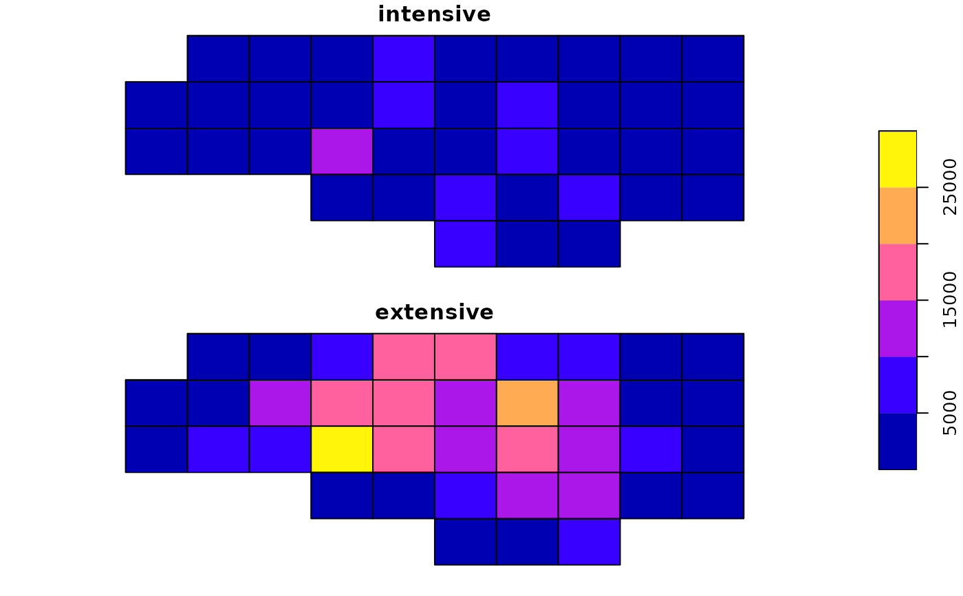
a1 = st_interpolate_aw(nc["BIR74"], g, extensive = FALSE)
#> Warning: st_interpolate_aw assumes attributes are constant or uniform over areas of x
sum(a1$BIR74) / sum(nc$BIR74) # not close to one: property is assumed spatially intensive
#> [1] 0.4026287
a2 = st_interpolate_aw(nc["BIR74"], g, extensive = TRUE)
#> Warning: st_interpolate_aw assumes attributes are constant or uniform over areas of x
# verify mass preservation (pycnophylactic) property:
sum(a2$BIR74) / sum(nc$BIR74)
#> [1] 0.9999998
a1$intensive = a1$BIR74
a1$extensive = a2$BIR74
plot(a1[c("intensive", "extensive")], key.pos = 4)
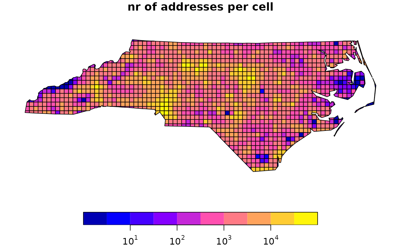
 # example Dasymetric mapping:
# load nr of addresses per 10 km grid cell, to proxy population -> birth density:
grd.addr = system.file("gpkg/grd_addr.gpkg", package="sf") |> read_sf()
nc = st_transform(nc, st_crs(grd.addr))
# avoid "assumes attributes are constant or uniform over areas" warnings:
st_agr(grd.addr) = c(ones = "constant")
st_agr(nc) = c(BIR74 = "constant", BIR79 = "constant")
plot(nc["BIR74"], logz = TRUE, main = "county birth counts, 1974-")
# example Dasymetric mapping:
# load nr of addresses per 10 km grid cell, to proxy population -> birth density:
grd.addr = system.file("gpkg/grd_addr.gpkg", package="sf") |> read_sf()
nc = st_transform(nc, st_crs(grd.addr))
# avoid "assumes attributes are constant or uniform over areas" warnings:
st_agr(grd.addr) = c(ones = "constant")
st_agr(nc) = c(BIR74 = "constant", BIR79 = "constant")
plot(nc["BIR74"], logz = TRUE, main = "county birth counts, 1974-")
 bir0.grd = st_interpolate_aw(nc[c("BIR74","BIR79")], extensive = TRUE, grd.addr)
plot(bir0.grd["BIR74"], logz = TRUE, main = "area-weighted birth counts, 1974-")
bir0.grd = st_interpolate_aw(nc[c("BIR74","BIR79")], extensive = TRUE, grd.addr)
plot(bir0.grd["BIR74"], logz = TRUE, main = "area-weighted birth counts, 1974-")
 xgrd.addr = grd.addr # copy for plotting
xgrd.addr$ones[grd.addr$ones==0] = 1 # so that logz shows finite values
plot(xgrd.addr, logz = TRUE, main = "nr of addresses per cell") # log scale
xgrd.addr = grd.addr # copy for plotting
xgrd.addr$ones[grd.addr$ones==0] = 1 # so that logz shows finite values
plot(xgrd.addr, logz = TRUE, main = "nr of addresses per cell") # log scale
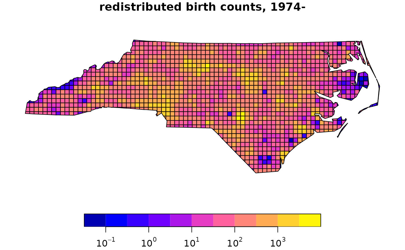
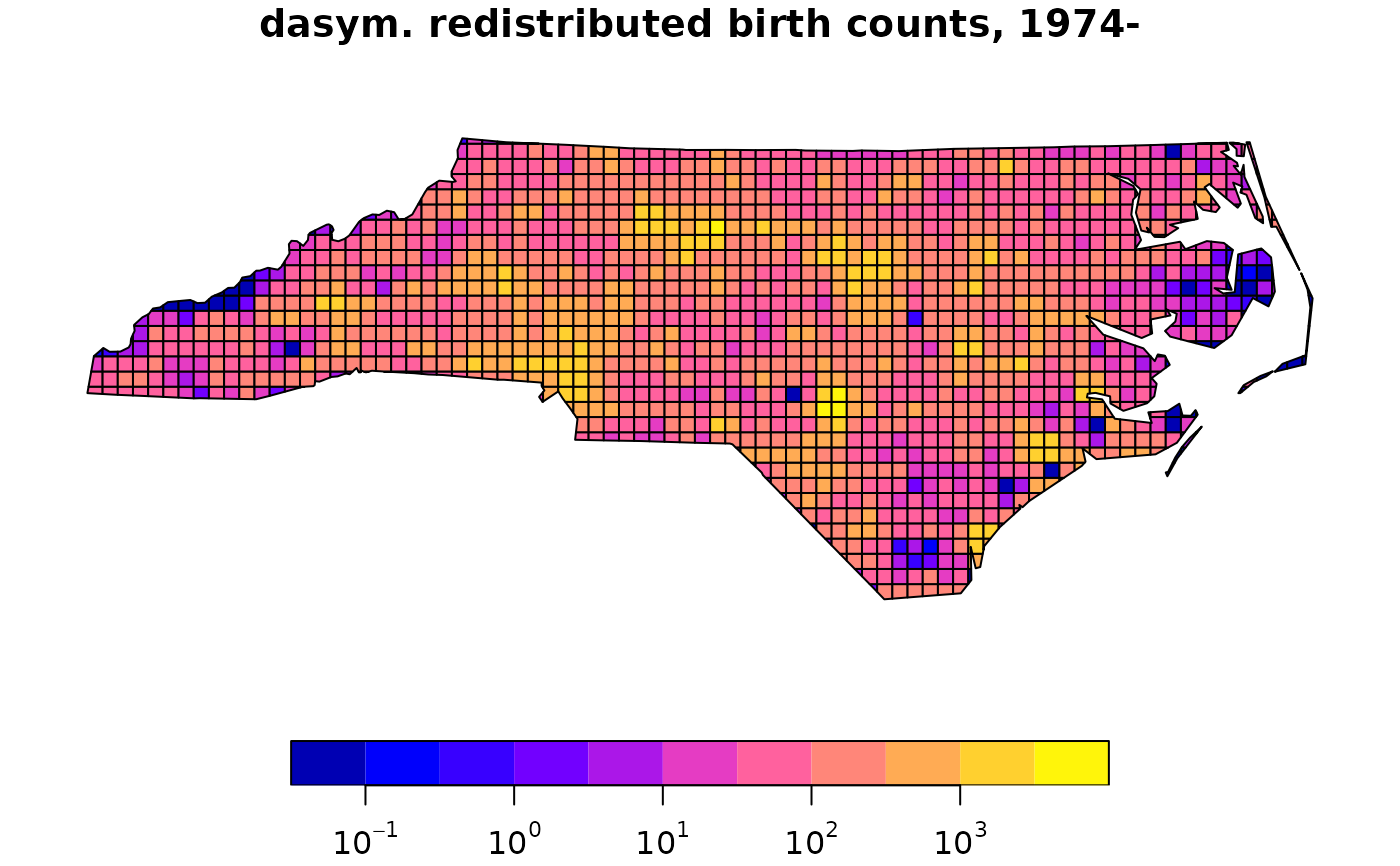
 # dasymetric mapping
bir.grd = st_interpolate_aw(nc[c("BIR74","BIR79")], extensive = TRUE, grd.addr, weights = "ones")
xbir.grd = bir.grd # copy for plotting
smallest_pos = function(x) min(x[x > 0])
xbir.grd$BIR74[xbir.grd$BIR74 == 0] = smallest_pos(xbir.grd$BIR74) # so that logz shows finite values
plot(xbir.grd["BIR74"], logz = TRUE, main = "dasym. redistributed birth counts, 1974-")
# dasymetric mapping
bir.grd = st_interpolate_aw(nc[c("BIR74","BIR79")], extensive = TRUE, grd.addr, weights = "ones")
xbir.grd = bir.grd # copy for plotting
smallest_pos = function(x) min(x[x > 0])
xbir.grd$BIR74[xbir.grd$BIR74 == 0] = smallest_pos(xbir.grd$BIR74) # so that logz shows finite values
plot(xbir.grd["BIR74"], logz = TRUE, main = "dasym. redistributed birth counts, 1974-")
 # verify sums:
apply(as.data.frame(bir.grd)[1:2], 2, sum)
#> BIR74 BIR79
#> 329962 422392
apply(as.data.frame(nc)[c("BIR74", "BIR79")], 2, sum)
#> BIR74 BIR79
#> 329962 422392
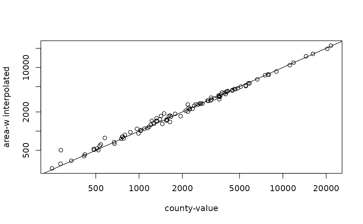
# compare county-wise:
st_agr(bir.grd) = c(BIR74 = "constant")
aw = st_interpolate_aw(bir.grd["BIR74"], st_geometry(nc), extensive = TRUE)
plot(nc$BIR74, aw$BIR74, log = 'xy', xlab = 'county-value', ylab = 'area-w interpolated')
abline(0,1)
# verify sums:
apply(as.data.frame(bir.grd)[1:2], 2, sum)
#> BIR74 BIR79
#> 329962 422392
apply(as.data.frame(nc)[c("BIR74", "BIR79")], 2, sum)
#> BIR74 BIR79
#> 329962 422392
# compare county-wise:
st_agr(bir.grd) = c(BIR74 = "constant")
aw = st_interpolate_aw(bir.grd["BIR74"], st_geometry(nc), extensive = TRUE)
plot(nc$BIR74, aw$BIR74, log = 'xy', xlab = 'county-value', ylab = 'area-w interpolated')
abline(0,1)