1. Simple Features for R

Simple features or simple feature access refers to a formal standard (ISO 19125-1:2004) that describes how objects in the real world can be represented in computers, with emphasis on the spatial geometry of these objects. It also describes how such objects can be stored in and retrieved from databases, and which geometrical operations should be defined for them.

The standard is widely implemented in spatial databases (such as PostGIS), commercial GIS (e.g., ESRI ArcGIS) and forms the vector data basis for libraries such as GDAL. A subset of simple features forms the GeoJSON standard.

R has well-supported classes for storing spatial data (sp) and interfacing to the above mentioned environments (rgdal, rgeos), but has so far lacked a complete implementation of simple features, making conversions at times convoluted, inefficient or incomplete. The package sf tries to fill this gap, and aims at succeeding sp in the long term.

This vignette:

explains what is meant by features, and by simple features
shows how they are implemented in R
provides examples of how you can work with them
shows how they can be read from and written to external files or resources (I/O)
discusses how they can be converted to and from sp objects
shows how they can be used for meaningful and applied spatial analysis

What is a feature?

A feature is thought of as a thing, or an object in the real world, such as a building or a tree. As is the case with objects, they often consist of other objects. This is the case with features too: a set of features can form a single feature. A forest stand can be a feature, a forest can be a feature, a city can be a feature. A satellite image pixel can be a feature, a complete image can be a feature too.

Features have a geometry describing where on Earth the feature is located, and they have attributes, which describe other properties. The geometry of a tree can be the delineation of its crown, of its stem, or the point indicating its centre. Other properties may include its height, color, diameter at breast height at a particular date, and so on.

The standard says: “A simple feature is defined by the OpenGIS Abstract specification to have both spatial and non-spatial attributes. Spatial attributes are geometry valued, and simple features are based on 2D geometry with linear interpolation between vertices.” We will see soon that the same standard will extend its coverage beyond 2D and beyond linear interpolation. Here, we take simple features as the data structures and operations described in the standard.

Dimensions

All geometries are composed of points. Points are coordinates in a 2-, 3- or 4-dimensional space. All points in a geometry have the same dimensionality. In addition to X and Y coordinates, there are two optional additional dimensions:

a Z coordinate, denoting altitude
an M coordinate (rarely used), denoting some measure that is associated with the point, rather than with the feature as a whole (in which case it would be a feature attribute); examples could be time of measurement, or measurement error of the coordinates

The four possible cases then are:

two-dimensional points refer to x and y, easting and northing, or longitude and latitude, we refer to them as XY
three-dimensional points as XYZ
three-dimensional points as XYM
four-dimensional points as XYZM (the third axis is Z, fourth M)

Simple feature geometry types

The following seven simple feature types are the most common, and are for instance the only ones used for GeoJSON:

type	description
`POINT`	zero-dimensional geometry containing a single point
`LINESTRING`	sequence of points connected by straight, non-self intersecting line pieces; one-dimensional geometry
`POLYGON`	geometry with a positive area (two-dimensional); sequence of points form a closed, non-self intersecting ring; the first ring denotes the exterior ring, zero or more subsequent rings denote holes in this exterior ring
`MULTIPOINT`	set of points; a MULTIPOINT is simple if no two Points in the MULTIPOINT are equal
`MULTILINESTRING`	set of linestrings
`MULTIPOLYGON`	set of polygons
`GEOMETRYCOLLECTION`	set of geometries of any type except GEOMETRYCOLLECTION

Each of the geometry types can also be a (typed) empty set, containing zero coordinates (for POINT the standard is not clear how to represent the empty geometry). Empty geometries can be thought of being the analogue to missing (NA) attributes, NULL values or empty lists.

The remaining geometries 10 are rarer, but increasingly find implementations:

type	description
`CIRCULARSTRING`	The CIRCULARSTRING is the basic curve type, similar to a LINESTRING in the linear world. A single segment requires three points, the start and end points (first and third) and any other point on the arc. The exception to this is for a closed circle, where the start and end points are the same. In this case the second point MUST be the center of the arc, i.e., the opposite side of the circle. To chain arcs together, the last point of the previous arc becomes the first point of the next arc, just like in LINESTRING. This means that a valid circular string must have an odd number of points greater than 1.
`COMPOUNDCURVE`	A compound curve is a single, continuous curve that has both curved (circular) segments and linear segments. That means that in addition to having well-formed components, the end point of every component (except the last) must be coincident with the start point of the following component.
`CURVEPOLYGON`	Example compound curve in a curve polygon: CURVEPOLYGON(COMPOUNDCURVE(CIRCULARSTRING(0 0,2 0, 2 1, 2 3, 4 3),(4 3, 4 5, 1 4, 0 0)), CIRCULARSTRING(1.7 1, 1.4 0.4, 1.6 0.4, 1.6 0.5, 1.7 1) )
`MULTICURVE`	A MultiCurve is a 1-dimensional GeometryCollection whose elements are Curves, it can include linear strings, circular strings or compound strings.
`MULTISURFACE`	A MultiSurface is a 2-dimensional GeometryCollection whose elements are Surfaces, all using coordinates from the same coordinate reference system.
`CURVE`	A Curve is a 1-dimensional geometric object usually stored as a sequence of Points, with the subtype of Curve specifying the form of the interpolation between Points
`SURFACE`	A Surface is a 2-dimensional geometric object
`POLYHEDRALSURFACE`	A PolyhedralSurface is a contiguous collection of polygons, which share common boundary segments
`TIN`	A TIN (triangulated irregular network) is a PolyhedralSurface consisting only of Triangle patches.
`TRIANGLE`	A Triangle is a polygon with 3 distinct, non-collinear vertices and no interior boundary

Note that CIRCULASTRING, COMPOUNDCURVE and CURVEPOLYGON are not described in the SFA standard, but in the SQL-MM part 3 standard. The descriptions above were copied from the PostGIS manual.

Coordinate reference system

Coordinates can only be placed on the Earth’s surface when their coordinate reference system (CRS) is known; this may be a spheroid CRS such as WGS84, a projected, two-dimensional (Cartesian) CRS such as a UTM zone or Web Mercator, or a CRS in three-dimensions, or including time. Similarly, M-coordinates need an attribute reference system, e.g. a measurement unit.

How simple features in R are organized

Package sf represents simple features as native R objects. Similar to PostGIS, all functions and methods in sf that operate on spatial data are prefixed by st_, which refers to spatial type; this makes them easily findable by command-line completion. Simple features are implemented as R native data, using simple data structures (S3 classes, lists, matrix, vector). Typical use involves reading, manipulating and writing of sets of features, with attributes and geometries.

As attributes are typically stored in data.frame objects (or the very similar tbl_df), we will also store feature geometries in a data.frame column. Since geometries are not single-valued, they are put in a list-column, a list of length equal to the number of records in the data.frame, with each list element holding the simple feature geometry of that feature. The three classes used to represent simple features are:

sf, the table (data.frame) with feature attributes and feature geometries, which contains
sfc, the list-column with the geometries for each feature (record), which is composed of
sfg, the feature geometry of an individual simple feature.

We will now discuss each of these three classes.

sf: objects with simple features

As we usually do not work with geometries of single simple features, but with datasets consisting of sets of features with attributes, the two are put together in sf (simple feature) objects. The following command reads the nc dataset from a file that is contained in the sf package:

library(sf)
## Linking to GEOS 3.10.2, GDAL 3.4.1, PROJ 8.2.1; sf_use_s2() is TRUE
nc <- st_read(system.file("shape/nc.shp", package="sf"))
## Reading layer `nc' from data source 
##   `/home/runner/work/_temp/Library/sf/shape/nc.shp' using driver `ESRI Shapefile'
## Simple feature collection with 100 features and 14 fields
## Geometry type: MULTIPOLYGON
## Dimension:     XY
## Bounding box:  xmin: -84.32385 ymin: 33.88199 xmax: -75.45698 ymax: 36.58965
## Geodetic CRS:  NAD27

(Note that users will not use system.file() but give a filename directly, and that shapefiles consist of more than one file, all with identical basename, which reside in the same directory.) The short report printed gives the file name, the driver (ESRI Shapefile), mentions that there are 100 features (records, represented as rows) and 14 fields (attributes, represented as columns). This object is of class

class(nc)
## [1] "sf"         "data.frame"

meaning it extends (and “is” a) data.frame, but with a single list-column with geometries, which is held in the column with name

attr(nc, "sf_column")
## [1] "geometry"

If we print the first three features, we see their attribute values and an abridged version of the geometry

print(nc[9:15], n = 3)

which would give the following output:

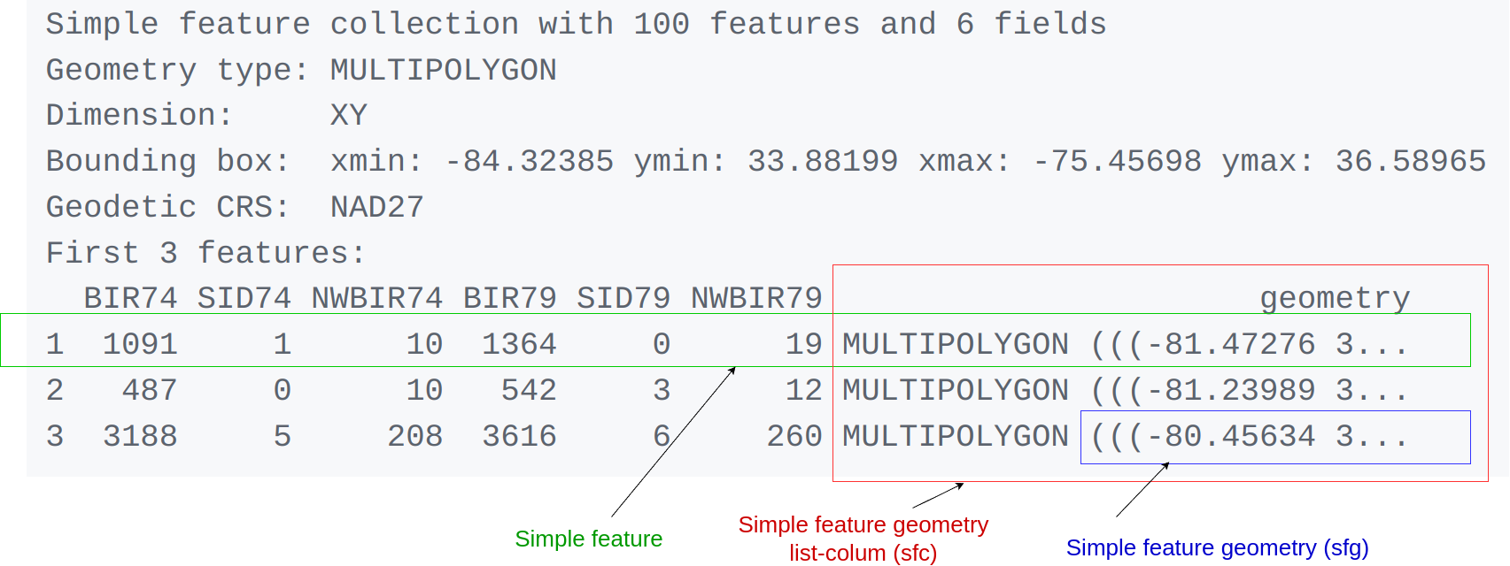
In the output we see:

in green a simple feature: a single record, or data.frame row, consisting of attributes and geometry
in blue a single simple feature geometry (an object of class sfg)
in red a simple feature list-column (an object of class sfc, which is a column in the data.frame)
that although geometries are native R objects, they are printed as well-known text

Methods for sf objects are:

methods(class = "sf")
##  [1] [                            [[<-                        
##  [3] [<-                          $<-                         
##  [5] aggregate                    as.data.frame               
##  [7] cbind                        coerce                      
##  [9] dbDataType                   dbWriteTable                
## [11] duplicated                   identify                    
## [13] initialize                   merge                       
## [15] plot                         points                      
## [17] print                        rbind                       
## [19] show                         slotsFromS3                 
## [21] st_agr                       st_agr<-                    
## [23] st_area                      st_as_s2                    
## [25] st_as_sf                     st_as_sfc                   
## [27] st_bbox                      st_boundary                 
## [29] st_break_antimeridian        st_buffer                   
## [31] st_cast                      st_centroid                 
## [33] st_collection_extract        st_concave_hull             
## [35] st_convex_hull               st_coordinates              
## [37] st_crop                      st_crs                      
## [39] st_crs<-                     st_difference               
## [41] st_drop_geometry             st_exterior_ring            
## [43] st_filter                    st_geometry                 
## [45] st_geometry<-                st_inscribed_circle         
## [47] st_interpolate_aw            st_intersection             
## [49] st_intersects                st_is_full                  
## [51] st_is_valid                  st_is                       
## [53] st_join                      st_line_merge               
## [55] st_m_range                   st_make_valid               
## [57] st_minimum_bounding_circle   st_minimum_rotated_rectangle
## [59] st_nearest_points            st_node                     
## [61] st_normalize                 st_point_on_surface         
## [63] st_polygonize                st_precision                
## [65] st_reverse                   st_sample                   
## [67] st_segmentize                st_set_precision            
## [69] st_shift_longitude           st_simplify                 
## [71] st_snap                      st_sym_difference           
## [73] st_transform                 st_triangulate_constrained  
## [75] st_triangulate               st_union                    
## [77] st_voronoi                   st_wrap_dateline            
## [79] st_write                     st_z_range                  
## [81] st_zm                        text                        
## [83] transform                   
## see '?methods' for accessing help and source code

It is also possible to create data.frame objects with geometry list-columns that are not of class sf, e.g. by:

nc.no_sf <- as.data.frame(nc)
class(nc.no_sf)
## [1] "data.frame"

However, such objects:

no longer register which column is the geometry list-column
no longer have a plot method, and
lack all of the other dedicated methods listed above for class sf

sfc: simple feature geometry list-column

The column in the sf data.frame that contains the geometries is a list, of class sfc. We can retrieve the geometry list-column in this case by nc$geom or nc[[15]], but the more general way uses st_geometry():

(nc_geom <- st_geometry(nc))
## Geometry set for 100 features 
## Geometry type: MULTIPOLYGON
## Dimension:     XY
## Bounding box:  xmin: -84.32385 ymin: 33.88199 xmax: -75.45698 ymax: 36.58965
## Geodetic CRS:  NAD27
## First 5 geometries:
## MULTIPOLYGON (((-81.47276 36.23436, -81.54084 3...
## MULTIPOLYGON (((-81.23989 36.36536, -81.24069 3...
## MULTIPOLYGON (((-80.45634 36.24256, -80.47639 3...
## MULTIPOLYGON (((-76.00897 36.3196, -76.01735 36...
## MULTIPOLYGON (((-77.21767 36.24098, -77.23461 3...

Geometries are printed in abbreviated form, but we can view a complete geometry by selecting it, e.g. the first one by:

nc_geom[[1]]
## MULTIPOLYGON (((-81.47276 36.23436, -81.54084 36.27251, -81.56198 36.27359, -81.63306 36.34069, -81.74107 36.39178, -81.69828 36.47178, -81.7028 36.51934, -81.67 36.58965, -81.3453 36.57286, -81.34754 36.53791, -81.32478 36.51368, -81.31332 36.4807, -81.26624 36.43721, -81.26284 36.40504, -81.24069 36.37942, -81.23989 36.36536, -81.26424 36.35241, -81.32899 36.3635, -81.36137 36.35316, -81.36569 36.33905, -81.35413 36.29972, -81.36745 36.2787, -81.40639 36.28505, -81.41233 36.26729, -81.43104 36.26072, -81.45289 36.23959, -81.47276 36.23436)))

The way this is printed is called well-known text, and is part of the standards. The word MULTIPOLYGON is followed by three parentheses, because it can consist of multiple polygons, in the form of MULTIPOLYGON(POL1,POL2), where POL1 might consist of an exterior ring and zero or more interior rings, as of (EXT1,HOLE1,HOLE2). Sets of coordinates belonging to a single polygon are held together with parentheses, so we get ((crds_ext)(crds_hole1)(crds_hole2)) where crds_ is a comma-separated set of coordinates of a ring. This leads to the case above, where MULTIPOLYGON(((crds_ext))) refers to the exterior ring (1), without holes (2), of the first polygon (3) - hence three parentheses.

We can see there is a single polygon with no rings:

par(mar = c(0,0,1,0))
plot(nc[1], reset = FALSE) # reset = FALSE: we want to add to a plot with a legend
plot(nc[1,1], col = 'grey', add = TRUE)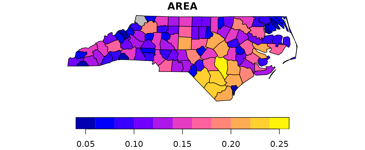

but some of the polygons in this dataset have multiple exterior rings; they can be identified by:

par(mar = c(0,0,1,0))
(w <- which(sapply(nc_geom, length) > 1))
## [1]  4 56 57 87 91 95
plot(nc[w,1], col = 2:7)

Following the MULTIPOLYGON datastructure, in R we have a list of lists of lists of matrices. For instance, we get the first 3 coordinate pairs of the second exterior ring (first ring is always exterior) for the geometry of feature 4 by:

nc_geom[[4]][[2]][[1]][1:3,]
##           [,1]     [,2]
## [1,] -76.02717 36.55672
## [2,] -75.99866 36.55665
## [3,] -75.91192 36.54253

Geometry columns have their own class,

class(nc_geom)
## [1] "sfc_MULTIPOLYGON" "sfc"

Methods for geometry list-columns include:

methods(class = 'sfc')
##  [1] [                            [<-                         
##  [3] as.data.frame                c                           
##  [5] coerce                       format                      
##  [7] identify                     initialize                  
##  [9] Ops                          points                      
## [11] print                        rep                         
## [13] show                         slotsFromS3                 
## [15] st_area                      st_as_binary                
## [17] st_as_grob                   st_as_s2                    
## [19] st_as_sf                     st_as_text                  
## [21] st_bbox                      st_boundary                 
## [23] st_break_antimeridian        st_buffer                   
## [25] st_cast                      st_centroid                 
## [27] st_collection_extract        st_concave_hull             
## [29] st_convex_hull               st_coordinates              
## [31] st_crop                      st_crs                      
## [33] st_crs<-                     st_difference               
## [35] st_exterior_ring             st_geometry                 
## [37] st_inscribed_circle          st_intersection             
## [39] st_intersects                st_is_full                  
## [41] st_is_valid                  st_is                       
## [43] st_line_merge                st_m_range                  
## [45] st_make_valid                st_minimum_bounding_circle  
## [47] st_minimum_rotated_rectangle st_nearest_points           
## [49] st_node                      st_normalize                
## [51] st_point_on_surface          st_polygonize               
## [53] st_precision                 st_reverse                  
## [55] st_sample                    st_segmentize               
## [57] st_set_precision             st_shift_longitude          
## [59] st_simplify                  st_snap                     
## [61] st_sym_difference            st_transform                
## [63] st_triangulate_constrained   st_triangulate              
## [65] st_union                     st_voronoi                  
## [67] st_wrap_dateline             st_write                    
## [69] st_z_range                   st_zm                       
## [71] str                          summary                     
## [73] text                         vec_cast.sfc                
## [75] vec_ptype2.sfc              
## see '?methods' for accessing help and source code

Coordinate reference systems (st_crs() and st_transform()) are discussed in the section on coordinate reference systems. st_as_wkb() and st_as_text() convert geometry list-columns into well-known-binary or well-known-text, explained below. st_bbox() retrieves the coordinate bounding box.

Attributes include:

attributes(nc_geom)
## $n_empty
## [1] 0
## 
## $crs
## Coordinate Reference System:
##   User input: NAD27 
##   wkt:
## GEOGCRS["NAD27",
##     DATUM["North American Datum 1927",
##         ELLIPSOID["Clarke 1866",6378206.4,294.978698213898,
##             LENGTHUNIT["metre",1]]],
##     PRIMEM["Greenwich",0,
##         ANGLEUNIT["degree",0.0174532925199433]],
##     CS[ellipsoidal,2],
##         AXIS["latitude",north,
##             ORDER[1],
##             ANGLEUNIT["degree",0.0174532925199433]],
##         AXIS["longitude",east,
##             ORDER[2],
##             ANGLEUNIT["degree",0.0174532925199433]],
##     ID["EPSG",4267]]
## 
## $class
## [1] "sfc_MULTIPOLYGON" "sfc"             
## 
## $precision
## [1] 0
## 
## $bbox
##      xmin      ymin      xmax      ymax 
## -84.32385  33.88199 -75.45698  36.58965

Mixed geometry types

The class of nc_geom is c("sfc_MULTIPOLYGON", "sfc"): sfc is shared with all geometry types, and sfc_TYPE with TYPE indicating the type of the particular geometry at hand.

There are two “special” types: GEOMETRYCOLLECTION, and GEOMETRY. GEOMETRYCOLLECTION indicates that each of the geometries may contain a mix of geometry types, as in

(mix <- st_sfc(st_geometrycollection(list(st_point(1:2))),
    st_geometrycollection(list(st_linestring(matrix(1:4,2))))))
## Geometry set for 2 features 
## Geometry type: GEOMETRYCOLLECTION
## Dimension:     XY
## Bounding box:  xmin: 1 ymin: 2 xmax: 2 ymax: 4
## CRS:           NA
## GEOMETRYCOLLECTION (POINT (1 2))
## GEOMETRYCOLLECTION (LINESTRING (1 3, 2 4))
class(mix)
## [1] "sfc_GEOMETRYCOLLECTION" "sfc"

Still, the geometries are here of a single type.

The second GEOMETRY, indicates that the geometries in the geometry list-column are of varying type:

(mix <- st_sfc(st_point(1:2), st_linestring(matrix(1:4,2))))
## Geometry set for 2 features 
## Geometry type: GEOMETRY
## Dimension:     XY
## Bounding box:  xmin: 1 ymin: 2 xmax: 2 ymax: 4
## CRS:           NA
## POINT (1 2)
## LINESTRING (1 3, 2 4)
class(mix)
## [1] "sfc_GEOMETRY" "sfc"

These two are fundamentally different: GEOMETRY is a superclass without instances, GEOMETRYCOLLECTION is a geometry instance. GEOMETRY list-columns occur when we read in a data source with a mix of geometry types. GEOMETRYCOLLECTION is a single feature’s geometry: the intersection of two feature polygons may consist of points, lines and polygons, see the example below.

sfg: simple feature geometry

Simple feature geometry (sfg) objects carry the geometry for a single feature, e.g. a point, linestring or polygon.

Simple feature geometries are implemented as R native data, using the following rules

a single POINT is a numeric vector
a set of points, e.g. in a LINESTRING or ring of a POLYGON is a matrix, each row containing a point
any other set is a list

Creator functions are rarely used in practice, since we typically bulk read and write spatial data. They are useful for illustration:

(x <- st_point(c(1,2)))
## POINT (1 2)
str(x)
##  'XY' num [1:2] 1 2
(x <- st_point(c(1,2,3)))
## POINT Z (1 2 3)
str(x)
##  'XYZ' num [1:3] 1 2 3
(x <- st_point(c(1,2,3), "XYM"))
## POINT M (1 2 3)
str(x)
##  'XYM' num [1:3] 1 2 3
(x <- st_point(c(1,2,3,4)))
## POINT ZM (1 2 3 4)
str(x)
##  'XYZM' num [1:4] 1 2 3 4
st_zm(x, drop = TRUE, what = "ZM")
## POINT (1 2)

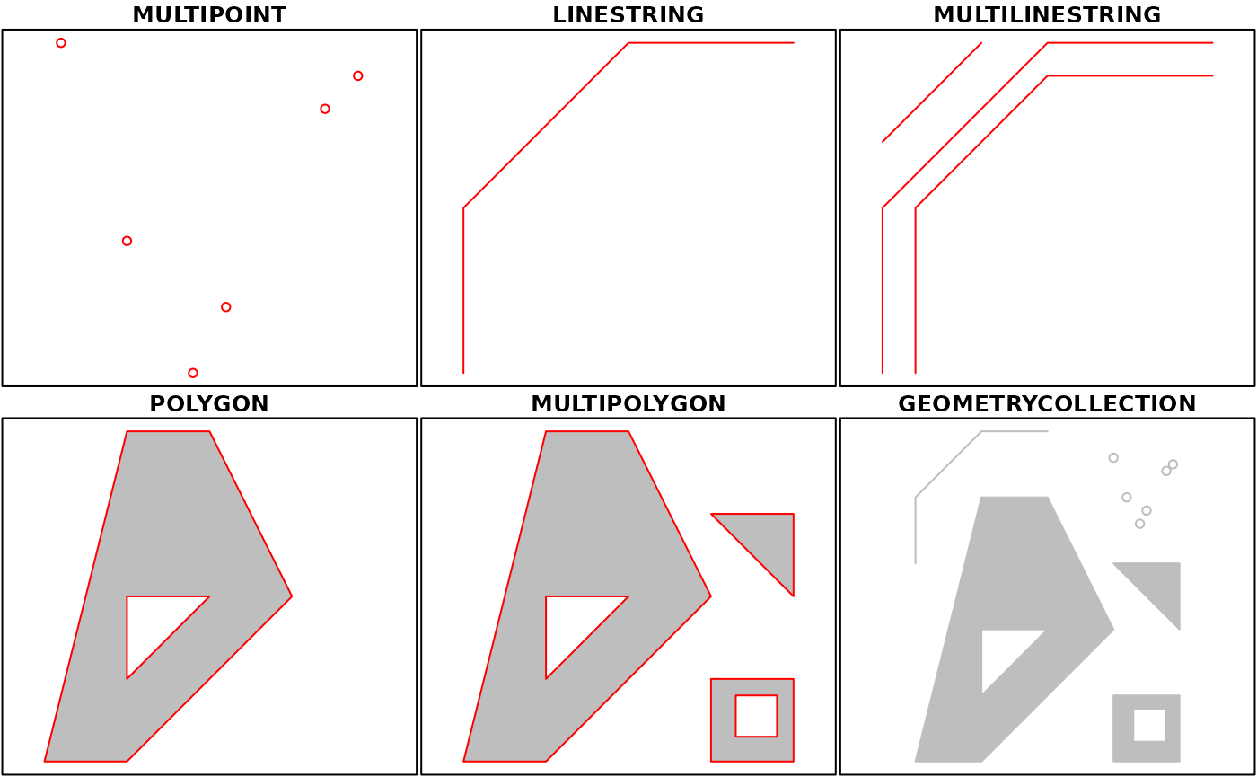
This means that we can represent 2-, 3- or 4-dimensional coordinates. All geometry objects inherit from sfg (simple feature geometry), but also have a type (e.g. POINT), and a dimension (e.g. XYM) class name. A figure illustrates six of the seven most common types.

With the exception of the POINT which has a single point as geometry, the remaining six common single simple feature geometry types that correspond to single features (single records, or rows in a data.frame) are created like this

p <- rbind(c(3.2,4), c(3,4.6), c(3.8,4.4), c(3.5,3.8), c(3.4,3.6), c(3.9,4.5))
(mp <- st_multipoint(p))
## MULTIPOINT ((3.2 4), (3 4.6), (3.8 4.4), (3.5 3.8), (3.4 3.6), (3.9 4.5))
s1 <- rbind(c(0,3),c(0,4),c(1,5),c(2,5))
(ls <- st_linestring(s1))
## LINESTRING (0 3, 0 4, 1 5, 2 5)
s2 <- rbind(c(0.2,3), c(0.2,4), c(1,4.8), c(2,4.8))
s3 <- rbind(c(0,4.4), c(0.6,5))
(mls <- st_multilinestring(list(s1,s2,s3)))
## MULTILINESTRING ((0 3, 0 4, 1 5, 2 5), (0.2 3, 0.2 4, 1 4.8, 2 4.8), (0 4.4, 0.6 5))
p1 <- rbind(c(0,0), c(1,0), c(3,2), c(2,4), c(1,4), c(0,0))
p2 <- rbind(c(1,1), c(1,2), c(2,2), c(1,1))
pol <-st_polygon(list(p1,p2))
p3 <- rbind(c(3,0), c(4,0), c(4,1), c(3,1), c(3,0))
p4 <- rbind(c(3.3,0.3), c(3.8,0.3), c(3.8,0.8), c(3.3,0.8), c(3.3,0.3))[5:1,]
p5 <- rbind(c(3,3), c(4,2), c(4,3), c(3,3))
(mpol <- st_multipolygon(list(list(p1,p2), list(p3,p4), list(p5))))
## MULTIPOLYGON (((0 0, 1 0, 3 2, 2 4, 1 4, 0 0), (1 1, 1 2, 2 2, 1 1)), ((3 0, 4 0, 4 1, 3 1, 3 0), (3.3 0.3, 3.3 0.8, 3.8 0.8, 3.8 0.3, 3.3 0.3)), ((3 3, 4 2, 4 3, 3 3)))
(gc <- st_geometrycollection(list(mp, mpol, ls)))
## GEOMETRYCOLLECTION (MULTIPOINT ((3.2 4), (3 4.6), (3.8 4.4), (3.5 3.8), (3.4 3.6), (3.9 4.5)), MULTIPOLYGON (((0 0, 1 0, 3 2, 2 4, 1 4, 0 0), (1 1, 1 2, 2 2, 1 1)), ((3 0, 4 0, 4 1, 3 1, 3 0), (3.3 0.3, 3.3 0.8, 3.8 0.8, 3.8 0.3, 3.3 0.3)), ((3 3, 4 2, 4 3, 3 3))), LINESTRING (0 3, 0 4, 1 5, 2 5))

The objects created are shown here:

Geometries can also be empty, as in

(x <- st_geometrycollection())
## GEOMETRYCOLLECTION EMPTY
length(x)
## [1] 0

Well-known text, well-known binary, precision

WKT and WKB

Well-known text (WKT) and well-known binary (WKB) are two encodings for simple feature geometries. Well-known text, e.g. seen in

x <- st_linestring(matrix(10:1,5))
st_as_text(x)
## [1] "LINESTRING (10 5, 9 4, 8 3, 7 2, 6 1)"

(but without the leading ## [1] and quotes), is human-readable. Coordinates are usually floating point numbers, and moving large amounts of information as text is slow and imprecise. For that reason, we use well-known binary (WKB) encoding

st_as_binary(x)
##  [1] 01 02 00 00 00 05 00 00 00 00 00 00 00 00 00 24 40 00 00 00 00 00 00 14 40
## [26] 00 00 00 00 00 00 22 40 00 00 00 00 00 00 10 40 00 00 00 00 00 00 20 40 00
## [51] 00 00 00 00 00 08 40 00 00 00 00 00 00 1c 40 00 00 00 00 00 00 00 40 00 00
## [76] 00 00 00 00 18 40 00 00 00 00 00 00 f0 3f

WKT and WKB can both be transformed back into R native objects by

st_as_sfc("LINESTRING(10 5, 9 4, 8 3, 7 2, 6 1)")[[1]]
## LINESTRING (10 5, 9 4, 8 3, 7 2, 6 1)
st_as_sfc(structure(list(st_as_binary(x)), class = "WKB"))[[1]]
## LINESTRING (10 5, 9 4, 8 3, 7 2, 6 1)

GDAL, GEOS, spatial databases and GIS read and write WKB which is fast and precise. Conversion between R native objects and WKB is done by package sf in compiled (C++/Rcpp) code, making this a reusable and fast route for I/O of simple feature geometries in R.

Precision

One of the attributes of a geometry list-column (sfc) is the precision: a double number that, when non-zero, causes some rounding during conversion to WKB, which might help certain geometrical operations succeed that would otherwise fail due to floating point representation. The model is that of GEOS, which copies from the Java Topology Suite (JTS), and works like this:

if precision is zero (default, unspecified), nothing is modified
negative values convert to float (4-byte real) precision
positive values convert to round(x*precision)/precision.

For the precision model, see also here, where it is written that: “… to specify 3 decimal places of precision, use a scale factor of 1000. To specify -3 decimal places of precision (i.e. rounding to the nearest 1000), use a scale factor of 0.001.” Note that all coordinates, so also Z or M values (if present) are affected. Choosing values for precision may require some experimenting.

Reading and writing

As we’ve seen above, reading spatial data from an external file can be done by:

filename <- system.file("shape/nc.shp", package="sf")
nc <- st_read(filename)
## Reading layer `nc' from data source 
##   `/home/runner/work/_temp/Library/sf/shape/nc.shp' using driver `ESRI Shapefile'
## Simple feature collection with 100 features and 14 fields
## Geometry type: MULTIPOLYGON
## Dimension:     XY
## Bounding box:  xmin: -84.32385 ymin: 33.88199 xmax: -75.45698 ymax: 36.58965
## Geodetic CRS:  NAD27

we can suppress the output by adding argument quiet=TRUE or by using the otherwise nearly identical but more quiet

nc <- read_sf(filename)

Writing takes place in the same fashion, using st_write():

st_write(nc, "nc.shp")
## Writing layer `nc' to data source `nc.shp' using driver `ESRI Shapefile'
## Writing 100 features with 14 fields and geometry type Multi Polygon.

If we repeat this, we get an error message that the file already exists, and we can overwrite by:

st_write(nc, "nc.shp", delete_layer = TRUE)
## Deleting layer `nc' using driver `ESRI Shapefile'
## Writing layer `nc' to data source `nc.shp' using driver `ESRI Shapefile'
## Writing 100 features with 14 fields and geometry type Multi Polygon.

or its quiet alternative that does this by default,

write_sf(nc, "nc.shp") # silently overwrites

Driver-specific options

The dsn and layer arguments to st_read() and st_write() denote a data source name and optionally a layer name. Their exact interpretation as well as the options they support vary per driver, the GDAL driver documentation is best consulted for this. For instance, a PostGIS table in database postgis might be read by:

meuse <- st_read("PG:dbname=postgis", "meuse")

where the PG: string indicates this concerns the PostGIS driver, followed by database name, and possibly port and user credentials. When the layer and driver arguments are not specified, st_read() tries to guess them from the datasource, or else simply reads the first layer, giving a warning in case there are more.

st_read() typically reads the coordinate reference system as proj4string, but not the EPSG (SRID). GDAL cannot retrieve SRID (EPSG code) from proj4string strings, and, when needed, it has to be set by the user. See also the section on coordinate reference systems.

st_drivers() returns a data.frame listing available drivers, and their metadata: names, whether a driver can write, and whether it is a raster and/or vector driver. All drivers can read. Reading of some common data formats is illustrated below:

st_layers(dsn) lists the layers present in data source dsn, and gives the number of fields, features and geometry type for each layer:

st_layers(system.file("osm/overpass.osm", package="sf"))

we see that in this case, the number of features is NA because for this xml file the whole file needs to be read, which may be costly for large files. We can force counting by:

Sys.setenv(OSM_USE_CUSTOM_INDEXING="NO")
st_layers(system.file("osm/overpass.osm", package="sf"), do_count = TRUE)

Another example of reading kml and kmz files is:

# Download .shp data
u_shp <- "http://coagisweb.cabq.gov/datadownload/biketrails.zip"
download.file(u_shp, "biketrails.zip")
unzip("biketrails.zip")
u_kmz <- "http://coagisweb.cabq.gov/datadownload/BikePaths.kmz"
download.file(u_kmz, "BikePaths.kmz")

# Read file formats
biketrails_shp <- st_read("biketrails.shp")
if(Sys.info()[1] == "Linux") # may not work if not Linux
  biketrails_kmz <- st_read("BikePaths.kmz")
u_kml = "http://www.northeastraces.com/oxonraces.com/nearme/safe/6.kml"
download.file(u_kml, "bikeraces.kml")
bikraces <- st_read("bikeraces.kml")

Create, read, update and delete

GDAL provides the crud (create, read, update, delete) functions to persistent storage. st_read() (or read_sf()) are used for reading. st_write() (or write_sf()) creates, and has the following arguments to control update and delete:

update=TRUE causes an existing data source to be updated, if it exists; this option is by default TRUE for all database drivers, where the database is updated by adding a table.
delete_layer=TRUE causes st_write try to open the data source and delete the layer; no errors are given if the data source is not present, or the layer does not exist in the data source.
delete_dsn=TRUE causes st_write to delete the data source when present, before writing the layer in a newly created data source. No error is given when the data source does not exist. This option should be handled with care, as it may wipe complete directories or databases.

Connection to spatial databases

Read and write functions, st_read() and st_write(), can handle connections to spatial databases to read WKB or WKT directly without using GDAL. Although intended to use the DBI interface, current use and testing of these functions are limited to PostGIS.

Coordinate reference systems and transformations

Coordinate reference systems (CRS) are like measurement units for coordinates: they specify which location on Earth a particular coordinate pair refers to. We saw above that sfc objects (geometry list-columns) have two attributes to store a CRS: epsg and proj4string. This implies that all geometries in a geometry list-column must have the same CRS. Both may be NA, e.g. in case the CRS is unknown, or when we work with local coordinate systems (e.g. inside a building, a body, or an abstract space).

proj4string is a generic, string-based description of a CRS, understood by the PROJ library. It defines projection types and (often) defines parameter values for particular projections, and hence can cover an infinite amount of different projections. This library (also used by GDAL) provides functions to convert or transform between different CRS. epsg is the integer ID for a particular, known CRS that can be resolved into a proj4string. Some proj4string values can resolved back into their corresponding epsg ID, but this does not always work.

The importance of having epsg values stored with data besides proj4string values is that the epsg refers to particular, well-known CRS, whose parameters may change (improve) over time; fixing only the proj4string may remove the possibility to benefit from such improvements, and limit some of the provenance of datasets, but may help reproducibility.

Coordinate reference system transformations can be carried out using st_transform(), e.g. converting longitudes/latitudes in NAD27 to web mercator (EPSG:3857) can be done by:

nc.web_mercator <- st_transform(nc, 3857)
st_geometry(nc.web_mercator)[[4]][[2]][[1]][1:3,]
##          [,1]    [,2]
## [1,] -8463267 4377519
## [2,] -8460094 4377510
## [3,] -8450437 4375553

Conversion, including to and from sp

sf objects and objects deriving from Spatial (package sp) can be coerced both ways:

showMethods("coerce", classes = "sf")
## Function: coerce (package methods)
## from="sf", to="Spatial"
## from="Spatial", to="sf"
methods(st_as_sf)
##  [1] st_as_sf.data.frame*   st_as_sf.lpp*          st_as_sf.map*         
##  [4] st_as_sf.owin*         st_as_sf.ppp*          st_as_sf.ppplist*     
##  [7] st_as_sf.psp*          st_as_sf.s2_geography* st_as_sf.sf*          
## [10] st_as_sf.sfc*          st_as_sf.Spatial*      st_as_sf.SpatVector*  
## see '?methods' for accessing help and source code
methods(st_as_sfc)
##  [1] st_as_sfc.bbox*               st_as_sfc.blob*              
##  [3] st_as_sfc.character*          st_as_sfc.dimensions*        
##  [5] st_as_sfc.factor*             st_as_sfc.list*              
##  [7] st_as_sfc.map*                st_as_sfc.owin*              
##  [9] st_as_sfc.pq_geometry*        st_as_sfc.psp*               
## [11] st_as_sfc.raw*                st_as_sfc.s2_geography*      
## [13] st_as_sfc.sf*                 st_as_sfc.SpatialLines*      
## [15] st_as_sfc.SpatialMultiPoints* st_as_sfc.SpatialPixels*     
## [17] st_as_sfc.SpatialPoints*      st_as_sfc.SpatialPolygons*   
## [19] st_as_sfc.tess*               st_as_sfc.WKB*               
## see '?methods' for accessing help and source code

# anticipate that sp::CRS will expand proj4strings:
p4s <- "+proj=longlat +datum=NAD27 +no_defs +ellps=clrk66 +nadgrids=@conus,@alaska,@ntv2_0.gsb,@ntv1_can.dat"
st_crs(nc) <- p4s

# anticipate geometry column name changes:
names(nc)[15] = "geometry"
attr(nc, "sf_column") = "geometry"
nc.sp <- as(nc, "Spatial")
class(nc.sp)
## [1] "SpatialPolygonsDataFrame"
## attr(,"package")
## [1] "sp"
nc2 <- st_as_sf(nc.sp)
all.equal(nc, nc2)
## [1] "Attributes: < Component \"class\": Lengths (4, 2) differ (string compare on first 2) >"           
## [2] "Attributes: < Component \"class\": 1 string mismatch >"                                           
## [3] "Component \"geometry\": Attributes: < Component \"crs\": Component \"input\": 1 string mismatch >"
## [4] "Component \"geometry\": Attributes: < Component \"crs\": Component \"wkt\": 1 string mismatch >"

As the Spatial* objects only support MULTILINESTRING and MULTIPOLYGON, LINESTRING and POLYGON geometries are automatically coerced into their MULTI form. When converting Spatial* into sf, if all geometries consist of a single POLYGON (possibly with holes), a POLYGON and otherwise all geometries are returned as MULTIPOLYGON: a mix of POLYGON and MULTIPOLYGON (such as common in shapefiles) is not created. Argument forceMulti=TRUE will override this, and create MULTIPOLYGONs in all cases. For LINES the situation is identical.

Geometrical operations

The standard for simple feature access defines a number of geometrical operations.

st_is_valid() and st_is_simple() return a Boolean indicating whether a geometry is valid or simple.

st_is_valid(nc[1:2,])
## [1] TRUE TRUE

st_distance() returns a dense numeric matrix with distances between geometries. st_relate() returns a character matrix with the DE9-IM values for each pair of geometries:

x = st_transform(nc, 32119)
st_distance(x[c(1,4,22),], x[c(1, 33,55,56),])
## Units: [m]
##           [,1]     [,2]      [,3]     [,4]
## [1,]      0.00 312184.9 128341.85 475623.3
## [2,] 440561.15 114939.7 590434.80      0.0
## [3,]  18944.03 352719.1  78756.89 517527.8
st_relate(nc[1:5,], nc[1:4,])
## although coordinates are longitude/latitude, st_relate assumes that they are
## planar
##      [,1]        [,2]        [,3]        [,4]       
## [1,] "2FFF1FFF2" "FF2F11212" "FF2FF1212" "FF2FF1212"
## [2,] "FF2F11212" "2FFF1FFF2" "FF2F11212" "FF2FF1212"
## [3,] "FF2FF1212" "FF2F11212" "2FFF1FFF2" "FF2FF1212"
## [4,] "FF2FF1212" "FF2FF1212" "FF2FF1212" "2FFF1FFF2"
## [5,] "FF2FF1212" "FF2FF1212" "FF2FF1212" "FF2FF1212"

st_intersects(), st_disjoint(), st_touches(), st_crosses(), st_within(), st_contains(), st_overlaps(), st_equals(), st_covers(), st_covered_by(), st_equals_exact() and st_is_within_distance() return a sparse matrix (sgbp object) with matching (TRUE) indexes, or a full logical matrix:

st_intersects(nc[1:5,], nc[1:4,])
## Sparse geometry binary predicate list of length 5, where the predicate
## was `intersects'
##  1: 1, 2
##  2: 1, 2, 3
##  3: 2, 3
##  4: 4
##  5: (empty)
st_intersects(nc[1:5,], nc[1:4,], sparse = FALSE)
##       [,1]  [,2]  [,3]  [,4]
## [1,]  TRUE  TRUE FALSE FALSE
## [2,]  TRUE  TRUE  TRUE FALSE
## [3,] FALSE  TRUE  TRUE FALSE
## [4,] FALSE FALSE FALSE  TRUE
## [5,] FALSE FALSE FALSE FALSE

st_buffer(), st_boundary(), st_convexhull(), st_union_cascaded, st_simplify, st_triangulate(), st_polygonize(), st_centroid(), st_segmentize(), and st_union() return new geometries, e.g.:

sel <- c(1,5,14)
geom = st_geometry(nc.web_mercator[sel,])
buf <- st_buffer(geom, dist = 30000)
plot(buf, border = 'red')
plot(geom, add = TRUE)
plot(st_buffer(geom, -5000), add = TRUE, border = 'blue')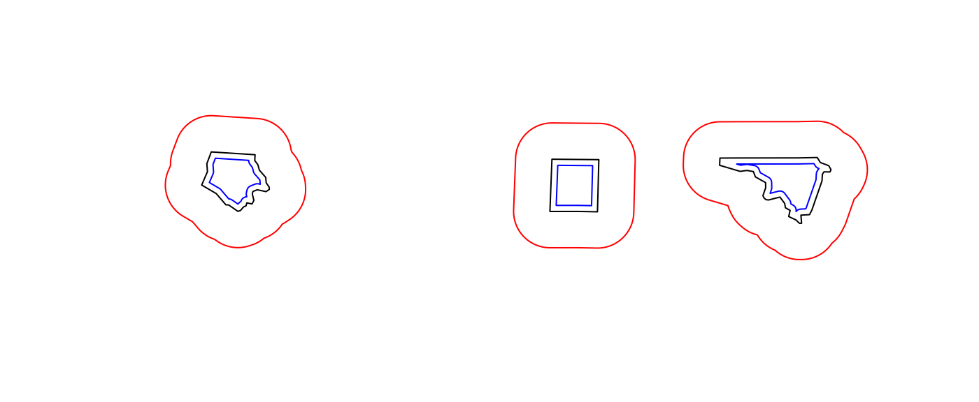

st_intersection(), st_union(), st_difference(), and st_sym_difference() return new geometries that are a function of pairs of geometries:

par(mar = rep(0,4))
u <- st_union(nc)
plot(u)

The following code shows how computing an intersection between two polygons may yield a GEOMETRYCOLLECTION with a point, line and polygon:

opar <- par(mfrow = c(1, 2))
a <- st_polygon(list(cbind(c(0,0,7.5,7.5,0),c(0,-1,-1,0,0))))
b <- st_polygon(list(cbind(c(0,1,2,3,4,5,6,7,7,0),c(1,0,.5,0,0,0.5,-0.5,-0.5,1,1))))
plot(a, ylim = c(-1,1))
title("intersecting two polygons:")
plot(b, add = TRUE, border = 'red')
(i <- st_intersection(a,b))
## GEOMETRYCOLLECTION (POLYGON ((7 0, 7 -0.5, 6 -0.5, 5.5 0, 7 0)), LINESTRING (4 0, 3 0), POINT (1 0))
plot(a, ylim = c(-1,1))
title("GEOMETRYCOLLECTION")
plot(b, add = TRUE, border = 'red')
plot(i, add = TRUE, col = 'green', lwd = 2)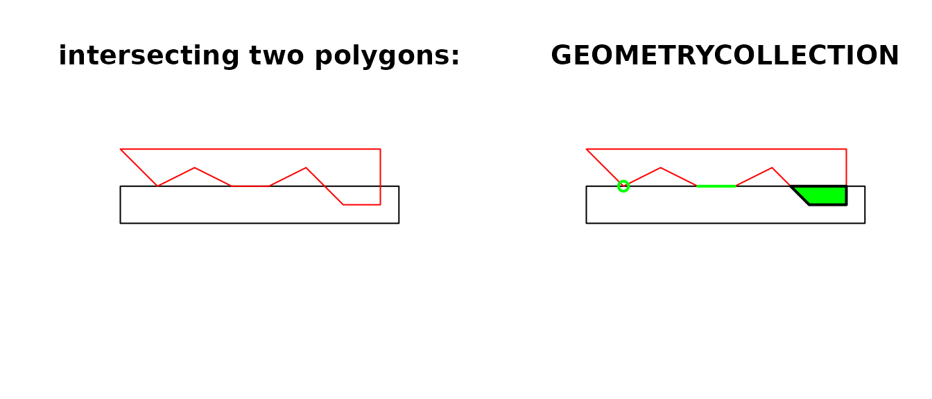

par(opar)

Non-simple and non-valid geometries

Non-simple geometries are for instance self-intersecting lines (left); non-valid geometries are for instance polygons with slivers (middle) or self-intersections (right).

library(sf)
x1 <- st_linestring(cbind(c(0,1,0,1),c(0,1,1,0)))
x2 <- st_polygon(list(cbind(c(0,1,1,1,0,0),c(0,0,1,0.6,1,0))))
x3 <- st_polygon(list(cbind(c(0,1,0,1,0),c(0,1,1,0,0))))
st_is_simple(st_sfc(x1))
## [1] FALSE
st_is_valid(st_sfc(x2,x3))
## [1] FALSE FALSE

Units

Where possible geometric operations such as st_distance(), st_length() and st_area() report results with a units attribute appropriate for the CRS:

a <- st_area(nc[1,])
attributes(a)
## $units
## $numerator
## [1] "m" "m"
## 
## $denominator
## character(0)
## 
## attr(,"class")
## [1] "symbolic_units"
## 
## $class
## [1] "units"

The units package can be used to convert between units:

units::set_units(a, km^2) # result in square kilometers
## 1137.108 [km^2]
units::set_units(a, ha) # result in hectares
## 113710.8 [ha]

The result can be stripped of their attributes if needs be:

as.numeric(a)
## [1] 1137107793

How attributes relate to geometries

(This will eventually be the topic of a new vignette; now here to explain the last attribute of sf objects)

The standard documents about simple features are very detailed about the geometric aspects of features, but say nearly nothing about attributes, except that their values should be understood in another reference system (their units of measurement, e.g. as implemented in the package units). But there is more to it. For variables like air temperature, interpolation usually makes sense, for others like human body temperature it doesn’t. The difference is that air temperature is a field, which continues between sensors, where body temperature is an object property that doesn’t extend beyond the body – in spatial statistics bodies would be called a point pattern, their temperature the point marks. For geometries that have a non-zero size (positive length or area), attribute values may refer to the every sub-geometry (every point), or may summarize the geometry. For example, a state’s population density summarizes the whole state, and is not a meaningful estimate of population density for a give point inside the state without the context of the state. On the other hand, land use or geological maps give polygons with constant land use or geology, every point inside the polygon is of that class. Some properties are spatially extensive, meaning that attributes would summed up when two geometries are merged: population is an example. Other properties are spatially intensive, and should be averaged, with population density the example.

Simple feature objects of class sf have an agr attribute that points to the attribute-geometry-relationship, how attributes relate to their geometry. It can be defined at creation time:

nc <- st_read(system.file("shape/nc.shp", package="sf"),
    agr = c(AREA = "aggregate", PERIMETER = "aggregate", CNTY_ = "identity",
        CNTY_ID = "identity", NAME = "identity", FIPS = "identity", FIPSNO = "identity",
        CRESS_ID = "identity", BIR74 = "aggregate", SID74 = "aggregate", NWBIR74 = "aggregate",
        BIR79 = "aggregate", SID79 = "aggregate", NWBIR79 = "aggregate"))
## Reading layer `nc' from data source 
##   `/home/runner/work/_temp/Library/sf/shape/nc.shp' using driver `ESRI Shapefile'
## Simple feature collection with 100 features and 14 fields
## Attribute-geometry relationships: aggregate (8), identity (6)
## Geometry type: MULTIPOLYGON
## Dimension:     XY
## Bounding box:  xmin: -84.32385 ymin: 33.88199 xmax: -75.45698 ymax: 36.58965
## Geodetic CRS:  NAD27
st_agr(nc)
##      AREA PERIMETER     CNTY_   CNTY_ID      NAME      FIPS    FIPSNO  CRESS_ID 
## aggregate aggregate  identity  identity  identity  identity  identity  identity 
##     BIR74     SID74   NWBIR74     BIR79     SID79   NWBIR79 
## aggregate aggregate aggregate aggregate aggregate aggregate 
## Levels: constant aggregate identity
data(meuse, package = "sp")
meuse_sf <- st_as_sf(meuse, coords = c("x", "y"), crs = 28992, agr = "constant")
st_agr(meuse_sf)
##  cadmium   copper     lead     zinc     elev     dist       om    ffreq 
## constant constant constant constant constant constant constant constant 
##     soil     lime  landuse   dist.m 
## constant constant constant constant 
## Levels: constant aggregate identity

When not specified, this field is filled with NA values, but if non-NA, it has one of three possibilities:

value	meaning
constant	a variable that has a constant value at every location over a spatial extent; examples: soil type, climate zone, land use
aggregate	values are summary values (aggregates) over the geometry, e.g. population density, dominant land use
identity	values identify the geometry: they refer to (the whole of) this and only this geometry

With this information (still to be done) we can for instance

either return missing values or generate warnings when a aggregate value at a point location inside a polygon is retrieved, or
list the implicit assumptions made when retrieving attribute values at points inside a polygon when relation_to_geometry is missing.
decide what to do with attributes when a geometry is split: do nothing in case the attribute is constant, give an error or warning in case it is an aggregate, change the relation_to_geometry to constant in case it was identity.

Edzer Pebesma