This vignette describes how simple features can be read in R from files or databases, and how they can be converted to other formats (text, sp)
Reading and writing through GDAL
The Geospatial Data Abstraction Library (GDAL) is the Swiss Army Knife for spatial
data: it reads and writes vector and raster data from and to practically
every file format, or database, of significance. Package sf
reads and writes using GDAL using st_read() and
st_write().
The data model GDAL uses needs
- a data source, which may be a file, directory, or database
- a layer, which is a single geospatial dataset inside a file or directory or e.g. a table in a database.
- the specification of a driver (i.e., which format)
- driver-specific reading or writing data sources, or layers
This may sound complex, but it is needed to map to over 200 data
formats! Package sf tries hard to simplify this where
possible (e.g. a file contains a single layer), but this vignette will
try to point you to the options.
Using st_read
As an example, we read the North Carolina counties SIDS dataset,
which comes shipped with the sf package by:
library(sf)
## Linking to GEOS 3.12.1, GDAL 3.8.4, PROJ 9.4.0; sf_use_s2() is TRUE
fname <- system.file("shape/nc.shp", package="sf")
fname
## [1] "/home/runner/work/_temp/Library/sf/shape/nc.shp"
nc <- st_read(fname)
## Reading layer `nc' from data source
##   `/home/runner/work/_temp/Library/sf/shape/nc.shp' using driver `ESRI Shapefile'
## Simple feature collection with 100 features and 14 fields
## Geometry type: MULTIPOLYGON
## Dimension:     XY
## Bounding box:  xmin: -84.32385 ymin: 33.88199 xmax: -75.45698 ymax: 36.58965
## Geodetic CRS:  NAD27
Typical users will use a file name with path for fname,
or first set R’s working directory with setwd() and use
file name without path.
We see here that a single argument is used to find both the datasource and the layer. This works when the datasource contains a single layer. In case the number of layers is zero (e.g. a database with no tables), an error message is given. In case there are more layers than one, the first layer is returned, but a message and a warning are given:
> st_read("PG:dbname=postgis")
Multiple layers are present in data source PG:dbname=postgis, reading layer `meuse'.
Use `st_layers' to list all layer names and their type in a data source.
Set the `layer' argument in `st_read' to read a particular layer.
Reading layer `meuse' from data source `PG:dbname=postgis' using driver `PostgreSQL'
Simple feature collection with 155 features and 12 fields
geometry type:  POINT
dimension:      XY
bbox:           xmin: 178605 ymin: 329714 xmax: 181390 ymax: 333611
epsg (SRID):    28992
proj4string:    +proj=sterea +lat_0=52.15616055555555 ...
Warning message:
In eval(substitute(expr), envir, enclos) :
  automatically selected the first layer in a data source containing more than one.
The message points to the st_layers() command, which
lists the driver and layers in a datasource, e.g.
> st_layers("PG:dbname=postgis")
Driver: PostgreSQL
Available layers:
  layer_name geometry_type features fields
1      meuse         Point      155     12
2   meuse_sf         Point      155     12
3       sids Multi Polygon      100     14
4  meuse_tbl         Point      155     13
5 meuse_tbl2         Point      155     13
>
A particular layer can now be read by e.g.
st_read("PG:dbname=postgis", "sids")st_layers() has the option to count the number of
features in case these are missing: some datasources (e.g. OSM xml
files) do not report the number of features, but need to be completely
read for this. GDAL allows for more than one geometry column for a
feature layer; these are reported by st_layers().
In case a layer contains only geometries but no attributes (fields),
st_read() still returns an sf object, with a
geometry column only.
We see that GDAL automatically detects the driver (file format) of the datasource, by trying them all in turn.
st_read() follows the conventions of base R, similar to
how it reads tabular data into data.frames. This means that
character data are read as character vectors by default
(since R 4.1.0). For those who insist on retrieving character data as
factors, the argument stringsAsFactors can be
set to TRUE:
st_read(fname, stringsAsFactors = TRUE)Alternatively, a user can set the global option
stringsAsFactors, and this will have the same effect:
options(stringsAsFactors = TRUE)
## Warning in options(stringsAsFactors = TRUE): 'options(stringsAsFactors = TRUE)'
## is deprecated and will be disabled
st_read(fname)
## Reading layer `nc' from data source
##   `/home/runner/work/_temp/Library/sf/shape/nc.shp' using driver `ESRI Shapefile'
## Simple feature collection with 100 features and 14 fields
## Geometry type: MULTIPOLYGON
## Dimension:     XY
## Bounding box:  xmin: -84.32385 ymin: 33.88199 xmax: -75.45698 ymax: 36.58965
## Geodetic CRS:  NAD27
Using st_write
To write a simple features object to a file, we need at least two arguments, the object and a filename:
st_write(nc, "nc1.shp")The file name is taken as the data source name. The default for the
layer name is the basename (filename without path) of the data source
name. For this, st_write() needs to guess the driver. The
above command is, for instance, equivalent to:
st_write(nc, dsn = "nc1.shp", layer = "nc.shp", driver = "ESRI Shapefile")
## Writing layer `nc' to data source `nc1.shp' using driver `ESRI Shapefile'
## Writing 100 features with 14 fields and geometry type Multi Polygon.
How the guessing of drivers works is explained in the next section.
Guessing a driver for output
The output driver is guessed from the datasource name, either from
its extension (.shp: ESRI Shapefile), or its
prefix (PG:: PostgreSQL). The list of
extensions with corresponding driver (short driver name) is:
| extension | driver short name |
|---|---|
bna |
BNA |
csv |
CSV |
e00 |
AVCE00 |
gdb |
FileGDB |
geojson |
GeoJSON |
gml |
GML |
gmt |
GMT |
gpkg |
GPKG |
gps |
GPSBabel |
gtm |
GPSTrackMaker |
gxt |
Geoconcept |
jml |
JML |
map |
WAsP |
mdb |
Geomedia |
nc |
netCDF |
ods |
ODS |
osm |
OSM |
pbf |
OSM |
shp |
ESRI Shapefile |
sqlite |
SQLite |
vdv |
VDV |
xls |
xls |
xlsx |
XLSX |
The list with prefixes is:
| prefix | driver short name |
|---|---|
couchdb: |
CouchDB |
DB2ODBC: |
DB2ODBC |
DODS: |
DODS |
GFT: |
GFT |
MSSQL: |
MSSQLSpatial |
MySQL: |
MySQL |
OCI: |
OCI |
ODBC: |
ODBC |
PG: |
PostgreSQL |
SDE: |
SDE |
Dataset and layer reading or creation options
Various GDAL drivers have options that influences the reading or writing process, for example what the driver should do when a table already exists in a database: append records to the table or overwrite it:
In case the table exists and the option is not specified, the driver
will give an error. Driver-specific options are documented in the driver
manual of gdal.
Multiple options can be given by multiple strings in
options.
For st_read(), there is only options; for
st_write(), one needs to distinguish between
dataset_options and layer_options, the first
related to opening a dataset, the second to creating layers in the
dataset.
Reading and writing directly to and from spatial databases
Package sf supports reading and writing from and to
spatial databases using the DBI interface. So far, testing
has mainly be done with PostGIS, other databases might work
but may also need more work. An example of reading is:
library(RPostgreSQL)
conn = dbConnect(PostgreSQL(), dbname = "postgis")
meuse = st_read(conn, "meuse")
meuse_1_3 = st_read(conn, query = "select * from meuse limit 3;")
dbDisconnect(conn)
We see here that in the second example a query is given. This query may contain spatial predicates, which could be a way to work through massive spatial datasets in R without having to read them completely in memory.
Similarly, tables can be written:
conn = dbConnect(PostgreSQL(), dbname = "postgis")
st_write(conn, meuse, drop = TRUE)
dbDisconnect(conn)
Here, the default table (layer) name is taken from the object name
(meuse). Argument drop informs to drop
(remove) the table before writing; logical argument binary
determines whether to use well-known binary or well-known text when
writing the geometry (where well-known binary is faster and
lossless).
Conversion to other formats: WKT, WKB, sp
Conversion to and from well-known text
The usual form in which we see simple features printed is well-known text:
st_point(c(0,1))
## POINT (0 1)
st_linestring(matrix(0:9,ncol=2,byrow=TRUE))
## LINESTRING (0 1, 2 3, 4 5, 6 7, 8 9)
We can create these well-known text strings explicitly using
st_as_text:
x = st_linestring(matrix(0:9,ncol=2,byrow=TRUE))
str = st_as_text(x)
x
## LINESTRING (0 1, 2 3, 4 5, 6 7, 8 9)
We can convert back from WKT by using st_as_sfc():
st_as_sfc(str)
## Geometry set for 1 feature
## Geometry type: LINESTRING
## Dimension:     XY
## Bounding box:  xmin: 0 ymin: 1 xmax: 8 ymax: 9
## CRS:           NA
## LINESTRING (0 1, 2 3, 4 5, 6 7, 8 9)
Conversion to and from well-known binary
Well-known binary is created from simple features by
st_as_binary():
x = st_linestring(matrix(0:9,ncol=2,byrow=TRUE))
(x = st_as_binary(x))
##  [1] 01 02 00 00 00 05 00 00 00 00 00 00 00 00 00 00 00 00 00 00 00 00 00 f0 3f
## [26] 00 00 00 00 00 00 00 40 00 00 00 00 00 00 08 40 00 00 00 00 00 00 10 40 00
## [51] 00 00 00 00 00 14 40 00 00 00 00 00 00 18 40 00 00 00 00 00 00 1c 40 00 00
## [76] 00 00 00 00 20 40 00 00 00 00 00 00 22 40
class(x)
## [1] "raw"
The object returned by st_as_binary() is of class
WKB and is either a list with raw vectors, or a single raw
vector. These can be converted into a hexadecimal character vector using
rawToHex():
rawToHex(x)
## [1] "0102000000050000000000000000000000000000000000f03f000000000000004000000000000008400000000000001040000000000000144000000000000018400000000000001c4000000000000020400000000000002240"
Converting back to sf uses st_as_sfc():
x = st_as_binary(st_sfc(st_point(0:1), st_point(5:6)))
st_as_sfc(x)
## Geometry set for 2 features
## Geometry type: POINT
## Dimension:     XY
## Bounding box:  xmin: 0 ymin: 1 xmax: 5 ymax: 6
## CRS:           NA
## POINT (0 1)
## POINT (5 6)
Conversion to and from sp
Spatial objects as maintained by package sp can be
converted into simple feature objects or geometries by
st_as_sf() and st_as_sfc(), respectively:
methods(st_as_sf)
##  [1] st_as_sf.data.frame*   st_as_sf.lpp*          st_as_sf.map*
##  [4] st_as_sf.owin*         st_as_sf.ppp*          st_as_sf.ppplist*
##  [7] st_as_sf.psp*          st_as_sf.s2_geography* st_as_sf.sf*
## [10] st_as_sf.sfc*          st_as_sf.Spatial*      st_as_sf.SpatVector*
## see '?methods' for accessing help and source code
methods(st_as_sfc)
##  [1] st_as_sfc.bbox*               st_as_sfc.blob*
##  [3] st_as_sfc.character*          st_as_sfc.dimensions*
##  [5] st_as_sfc.factor*             st_as_sfc.list*
##  [7] st_as_sfc.map*                st_as_sfc.owin*
##  [9] st_as_sfc.pq_geometry*        st_as_sfc.psp*
## [11] st_as_sfc.raw*                st_as_sfc.s2_geography*
## [13] st_as_sfc.sf*                 st_as_sfc.SpatialLines*
## [15] st_as_sfc.SpatialMultiPoints* st_as_sfc.SpatialPixels*
## [17] st_as_sfc.SpatialPoints*      st_as_sfc.SpatialPolygons*
## [19] st_as_sfc.tess*               st_as_sfc.WKB*
## see '?methods' for accessing help and source code
An example would be:
library(sp)
data(meuse)
coordinates(meuse) = ~x+y
m.sf = st_as_sf(meuse)
opar = par(mar=rep(0,4))
plot(m.sf)
## Warning: plotting the first 10 out of 12 attributes; use max.plot = 12 to plot
## all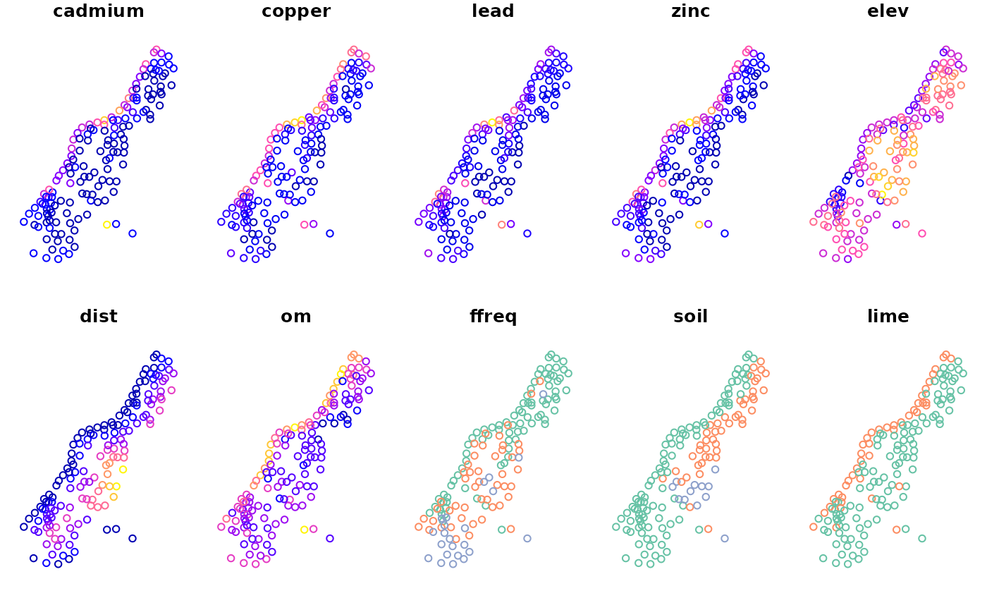
Conversion of simple feature objects of class sf or
sfc into corresponding Spatial* objects is
done using the as method, coercing to
Spatial: