plot sf object — plot • sf

plot one or more attributes of an sf object on a map Plot sf object

Usage

# S3 method for class 'sf'
plot(
  x,
  y,
  ...,
  main,
  pal = NULL,
  nbreaks = 10,
  breaks = "pretty",
  max.plot = getOption("sf_max.plot", default = 9),
  key.pos = get_key_pos(x, ...),
  key.length = 0.618,
  key.width = kw_dflt(x, key.pos),
  reset = TRUE,
  logz = FALSE,
  extent = x,
  xlim = st_bbox(extent)[c(1, 3)],
  ylim = st_bbox(extent)[c(2, 4)],
  compact = FALSE
)

get_key_pos(x, ...)

# S3 method for class 'sfc_POINT'
plot(
  x,
  y,
  ...,
  pch = 1,
  cex = 1,
  col = 1,
  bg = 0,
  lwd = 1,
  lty = 1,
  type = "p",
  add = FALSE
)

# S3 method for class 'sfc_MULTIPOINT'
plot(
  x,
  y,
  ...,
  pch = 1,
  cex = 1,
  col = 1,
  bg = 0,
  lwd = 1,
  lty = 1,
  type = "p",
  add = FALSE
)

# S3 method for class 'sfc_LINESTRING'
plot(x, y, ..., lty = 1, lwd = 1, col = 1, pch = 1, type = "l", add = FALSE)

# S3 method for class 'sfc_CIRCULARSTRING'
plot(x, y, ...)

# S3 method for class 'sfc_MULTILINESTRING'
plot(x, y, ..., lty = 1, lwd = 1, col = 1, pch = 1, type = "l", add = FALSE)

# S3 method for class 'sfc_POLYGON'
plot(
  x,
  y,
  ...,
  lty = 1,
  lwd = 1,
  col = NA,
  cex = 1,
  pch = NA,
  border = 1,
  add = FALSE,
  rule = "evenodd",
  xpd = par("xpd")
)

# S3 method for class 'sfc_MULTIPOLYGON'
plot(
  x,
  y,
  ...,
  lty = 1,
  lwd = 1,
  col = NA,
  border = 1,
  add = FALSE,
  rule = "evenodd",
  xpd = par("xpd")
)

# S3 method for class 'sfc_GEOMETRYCOLLECTION'
plot(
  x,
  y,
  ...,
  pch = 1,
  cex = 1,
  bg = 0,
  lty = 1,
  lwd = 1,
  col = 1,
  border = 1,
  add = FALSE
)

# S3 method for class 'sfc_GEOMETRY'
plot(
  x,
  y,
  ...,
  pch = 1,
  cex = 1,
  bg = 0,
  lty = 1,
  lwd = 1,
  col = ifelse(st_dimension(x) == 2, NA, 1),
  border = 1,
  add = FALSE
)

# S3 method for class 'sfg'
plot(x, ...)

plot_sf(
  x,
  xlim = NULL,
  ylim = NULL,
  asp = NA,
  axes = FALSE,
  bgc = par("bg"),
  ...,
  xaxs,
  yaxs,
  lab,
  setParUsrBB = FALSE,
  bgMap = NULL,
  expandBB = c(0, 0, 0, 0),
  graticule = NA_crs_,
  col_graticule = "grey",
  border,
  extent = x
)

sf.colors(n = 10, cutoff.tails = c(0.35, 0.2), alpha = 1, categorical = FALSE)

# S3 method for class 'sf'
text(x, labels = row.names(x), ...)

# S3 method for class 'sfc'
text(x, labels = seq_along(x), ..., of_largest_polygon = FALSE)

# S3 method for class 'sf'
points(x, ...)

# S3 method for class 'sfc'
points(x, ..., of_largest_polygon = FALSE)

Arguments

x: object of class sf
y: ignored
...: further specifications, see plot_sf and plot and details.
main: title for plot (NULL to remove)
pal: palette function, similar to rainbow, or palette values; if omitted, sf.colors is used
nbreaks: number of colors breaks (ignored for factor or character variables)
breaks: either a numeric vector with the actual breaks, or a name of a method accepted by the style argument of classIntervals
max.plot: integer; lower boundary to maximum number of attributes to plot; the default value (9) can be overridden by setting the global option sf_max.plot, e.g. options(sf_max.plot=2)
key.pos: numeric; side to plot a color key: 1 bottom, 2 left, 3 top, 4 right; set to NULL to omit key completely, 0 to only not plot the key, or -1 to select automatically. If multiple columns are plotted in a single function call by default no key is plotted and every submap is stretched individually; if a key is requested (and col is missing) all maps are colored according to a single key. Auto select depends on plot size, map aspect, and, if set, parameter asp. If it has lenght 2, the second value, ranging from 0 to 1, determines where the key is placed in the available space (default: 0.5, center).
key.length: amount of space reserved for the key along its axis, length of the scale bar
key.width: amount of space reserved for the key (incl. labels), thickness/width of the scale bar
reset: logical; if FALSE, keep the plot in a mode that allows adding further map elements; if TRUE restore original mode after plotting sf objects with attributes; see details.
logz: logical; if TRUE, use log10-scale for the attribute variable. In that case, breaks and at need to be given as log10-values; see examples.
extent: object with an st_bbox method to define plot extent; defaults to x
xlim: see plot.window
ylim: see plot.window
compact: logical; compact sub-plots over plotting space?
pch: plotting symbol
cex: symbol size
col: color for plotting features; if length(col) does not equal 1 or nrow(x), a warning is emitted that colors will be recycled. Specifying col suppresses plotting the legend key.
bg: symbol background color
lwd: line width
lty: line type
type: plot type: 'p' for points, 'l' for lines, 'b' for both
add: logical; add to current plot? Note that when using add=TRUE, you may have to set reset=FALSE in the first plot command.
border: color of polygon border(s); using NA hides them
rule: see polypath; for winding, exterior ring direction should be opposite that of the holes; with evenodd, plotting is robust against misspecified ring directions
xpd: see par; sets polygon clipping strategy; only implemented for POLYGON and MULTIPOLYGON
asp: see below, and see par
axes: logical; should axes be plotted? (default FALSE)
bgc: background color
xaxs: see par
yaxs: see par
lab: see par
setParUsrBB: default FALSE; set the par “usr” bounding box; see below
bgMap: object of class ggmap, or returned by function RgoogleMaps::GetMap
expandBB: numeric; fractional values to expand the bounding box with, in each direction (bottom, left, top, right)
graticule: logical, or object of class crs (e.g., st_crs(4326) for a WGS84 graticule), or object created by st_graticule; TRUE will give the WGS84 graticule or object returned by st_graticule
col_graticule: color to used for the graticule (if present)
n: integer; number of colors
cutoff.tails: numeric, in [0,0.5] start and end values
alpha: numeric, in [0,1], transparency
categorical: logical; do we want colors for a categorical variable? (see details)
labels: character, text to draw (one per row of input)
of_largest_polygon: logical, passed on to st_centroid

Details

plot.sf maximally plots max.plot maps with colors following from attribute columns, one map per attribute. It uses sf.colors for default colors. For more control over placement of individual maps, set parameter mfrow with par prior to plotting, and plot single maps one by one; note that this only works in combination with setting parameters key.pos=NULL (no legend) and reset=FALSE.

plot.sfc plots the geometry, additional parameters can be passed on to control color, lines or symbols.

When setting reset to FALSE, the original device parameters are lost, and the device must be reset using dev.off() in order to reset it.

parameter at can be set to specify where labels are placed along the key; see examples.

The features are plotted in the order as they apppear in the sf object. See examples for when a different plotting order is wanted.

plot_sf sets up the plotting area, axes, graticule, or webmap background; it is called by all plot methods before anything is drawn.

The argument setParUsrBB may be used to pass the logical value TRUE to functions within plot.Spatial. When set to TRUE, par(“usr”) will be overwritten with c(xlim, ylim), which defaults to the bounding box of the spatial object. This is only needed in the particular context of graphic output to a specified device with given width and height, to be matched to the spatial object, when using par(“xaxs”) and par(“yaxs”) in addition to par(mar=c(0,0,0,0)).

The default aspect for map plots is 1; if however data are not projected (coordinates are long/lat), the aspect is by default set to 1/cos(My * pi/180) with My the y coordinate of the middle of the map (the mean of ylim, which defaults to the y range of bounding box). This implies an Equirectangular projection.

non-categorical colors from sf.colors were taken from bpy.colors, with modified cutoff.tails defaults If categorical is TRUE, default colors are from https://colorbrewer2.org/ (if n < 9, Set2, else Set3).

text.sf adds text to an existing base graphic. Text is placed at the centroid of each feature in x. Provide POINT features for further control of placement. points.sf adds point symbols to an existing base graphic. If points of text are not shown correctly, try setting argument reset to FALSE in the plot() call.

Examples

nc = st_read(system.file("gpkg/nc.gpkg", package="sf"), quiet = TRUE)
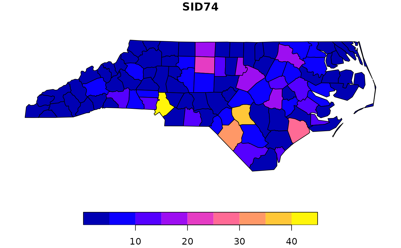
# plot single attribute, auto-legend:
plot(nc["SID74"])

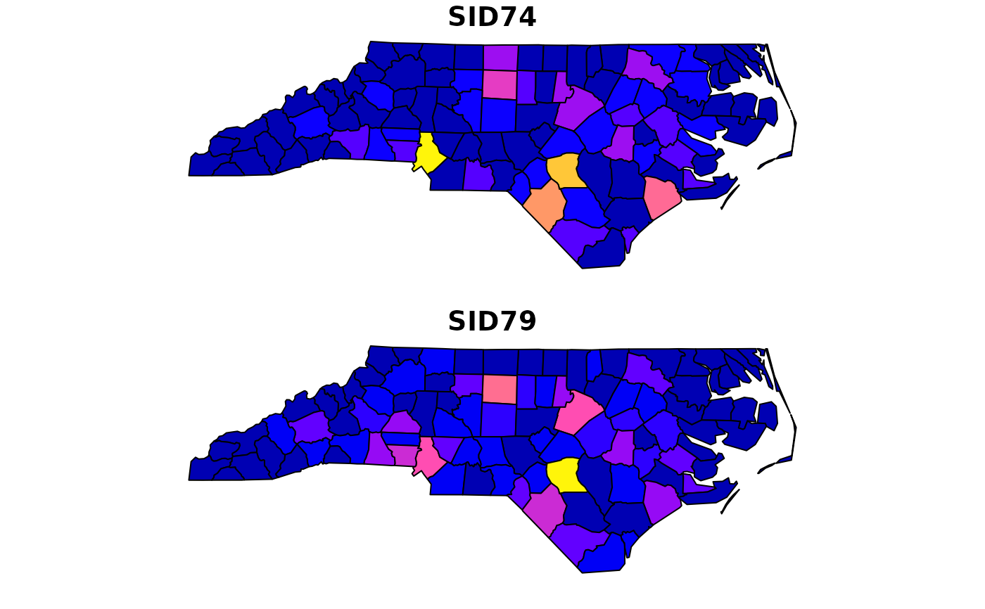
# plot multiple:
plot(nc[c("SID74", "SID79")]) # better use ggplot2::geom_sf to facet and get a single legend!

# adding to a plot of an sf object only works when using reset=FALSE in the first plot:
plot(nc["SID74"], reset = FALSE)
plot(st_centroid(st_geometry(nc)), add = TRUE)

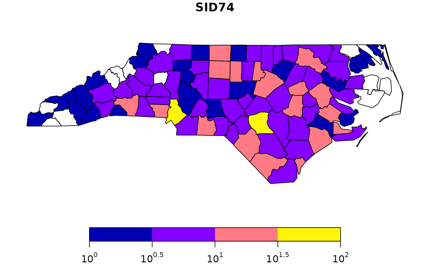
# log10 z-scale:
plot(nc["SID74"], logz = TRUE, breaks = c(0,.5,1,1.5,2), at = c(0,.5,1,1.5,2))

# and we need to reset the plotting device after that, e.g. by
layout(1)
# when plotting only geometries, the reset=FALSE is not needed:
plot(st_geometry(nc))
plot(st_geometry(nc)[1], col = 'red', add = TRUE)

# add a custom legend to an arbitray plot:
layout(matrix(1:2, ncol = 2), widths = c(1, lcm(2)))
plot(1)
.image_scale(1:10, col = sf.colors(9), key.length = lcm(8), key.pos = 4, at = 1:10)

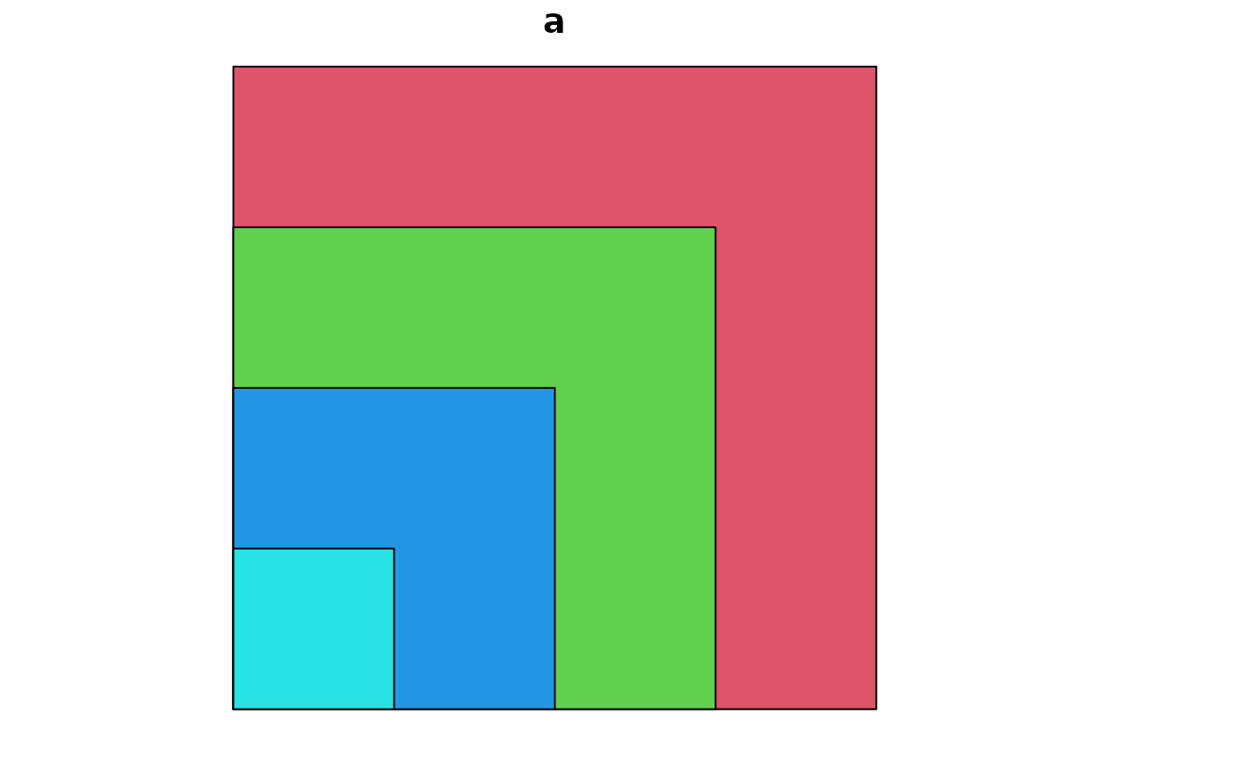
# manipulate plotting order, plot largest polygons first:
p = st_polygon(list(rbind(c(0,0), c(1,0), c(1,1), c(0,1), c(0,0))))
x = st_sf(a=1:4, st_sfc(p, p * 2, p * 3, p * 4)) # plot(x, col=2:5) only shows the largest polygon!
plot(x[order(st_area(x), decreasing = TRUE),], col = 2:5) # plot largest polygons first

sf.colors(10)
#>  [1] "#0000B3FF" "#0400FFFF" "#4500FFFF" "#8500FFFF" "#C527D8FF" "#FF50AFFF"
#>  [7] "#FF7A85FF" "#FFA35CFF" "#FFCC33FF" "#FFF50AFF"
text(nc, labels = substring(nc$NAME,1,1))