Graph based spatial weights

Functions return a graph object containing a list with the vertex coordinates and the to and from indices defining the edges. Some/all of these functions assume that the coordinates are not exactly regularly spaced. The helper function graph2nb converts a graph object into a neighbour list. The plot functions plot the graph objects.

gabrielneigh(coords, nnmult=3)
relativeneigh(coords, nnmult=3)
<!-- %beta.skel(coords,beta) -->
soi.graph(tri.nb, coords, quadsegs=10)
graph2nb(gob, row.names=NULL,sym=FALSE)
# S3 method for Gabriel
plot(x, show.points=FALSE, add=FALSE, linecol=par(col), ...)
# S3 method for relative
plot(x, show.points=FALSE, add=FALSE, linecol=par(col),...)

Arguments

coords: matrix of region point coordinates or SpatialPoints object or sfc points object
nnmult: scaling factor for memory allocation, default 3; if higher values are required, the function will exit with an error; example below thanks to Dan Putler
tri.nb: a neighbor list created from tri2nb
quadsegs: number of line segments making a quarter circle buffer, see the nQuadSegs argument in geos_unary

gob: a graph object created from any of the graph funtions
row.names: character vector of region ids to be added to the neighbours list as attribute region.id, default seq(1, nrow(x))
sym: a logical argument indicating whether or not neighbors should be symetric (if i->j then j->i)
x: object to be plotted
show.points: (logical) add points to plot
add: (logical) add to existing plot
linecol: edge plotting colour
...: further graphical parameters as in par(..)

Details

The graph functions produce graphs on a 2d point set that are all subgraphs of the Delaunay triangulation. The relative neighbor graph is defined by the relation, x and y are neighbors if

$$d(x,y) \le min(max(d(x,z),d(y,z))| z \in S)$$

where d() is the distance, S is the set of points and z is an arbitrary point in S. The Gabriel graph is a subgraph of the delaunay triangulation and has the relative neighbor graph as a sub-graph. The relative neighbor graph is defined by the relation x and y are Gabriel neighbors if

$$d(x,y) \le min((d(x,z)^2 + d(y,z)^2)^{1/2} |z \in S)$$

where x,y,z and S are as before. The sphere of influence graph is defined for a finite point set S, let $r_x$ be the distance from point x to its nearest neighbor in S, and $C_x$ is the circle centered on x. Then x and y are SOI neigbors iff $C_x$ and $C_y$ intersect in at least 2 places. From 2016-05-31, Computational Geometry in C code replaced by calls to functions in dbscan and sf; with a large quadsegs= argument, the behaviour of the function is the same, otherwise buffer intersections only closely approximate the original function.

See card for details of “nb” objects.

Value

A list of class Graph with the following elements

np: number of input points
from: array of origin ids
to: array of destination ids
nedges: number of edges in graph
x: input x coordinates
y: input y coordinates

The helper functions return an nb object with a list of integer vectors containing neighbour region number ids.

References

Matula, D. W. and Sokal R. R. 1980, Properties of Gabriel graphs relevant to geographic variation research and the clustering of points in the plane, Geographic Analysis, 12(3), pp. 205-222.

Toussaint, G. T. 1980, The relative neighborhood graph of a finite planar set, Pattern Recognition, 12(4), pp. 261-268.

Kirkpatrick, D. G. and Radke, J. D. 1985, A framework for computational morphology. In Computational Geometry, Ed. G. T. Toussaint, North Holland.

Author

Nicholas Lewin-Koh nikko@hailmail.net

Examples

columbus <- st_read(system.file("shapes/columbus.shp", package="spData")[1], quiet=TRUE)
sf_obj <- st_centroid(st_geometry(columbus), of_largest_polygon)
sp_obj <- as(sf_obj, "Spatial")
coords <- st_coordinates(sf_obj)
suppressMessages(col.tri.nb <- tri2nb(coords))
col.gab.nb <- graph2nb(gabrielneigh(coords), sym=TRUE)
col.rel.nb <- graph2nb(relativeneigh(coords), sym=TRUE)
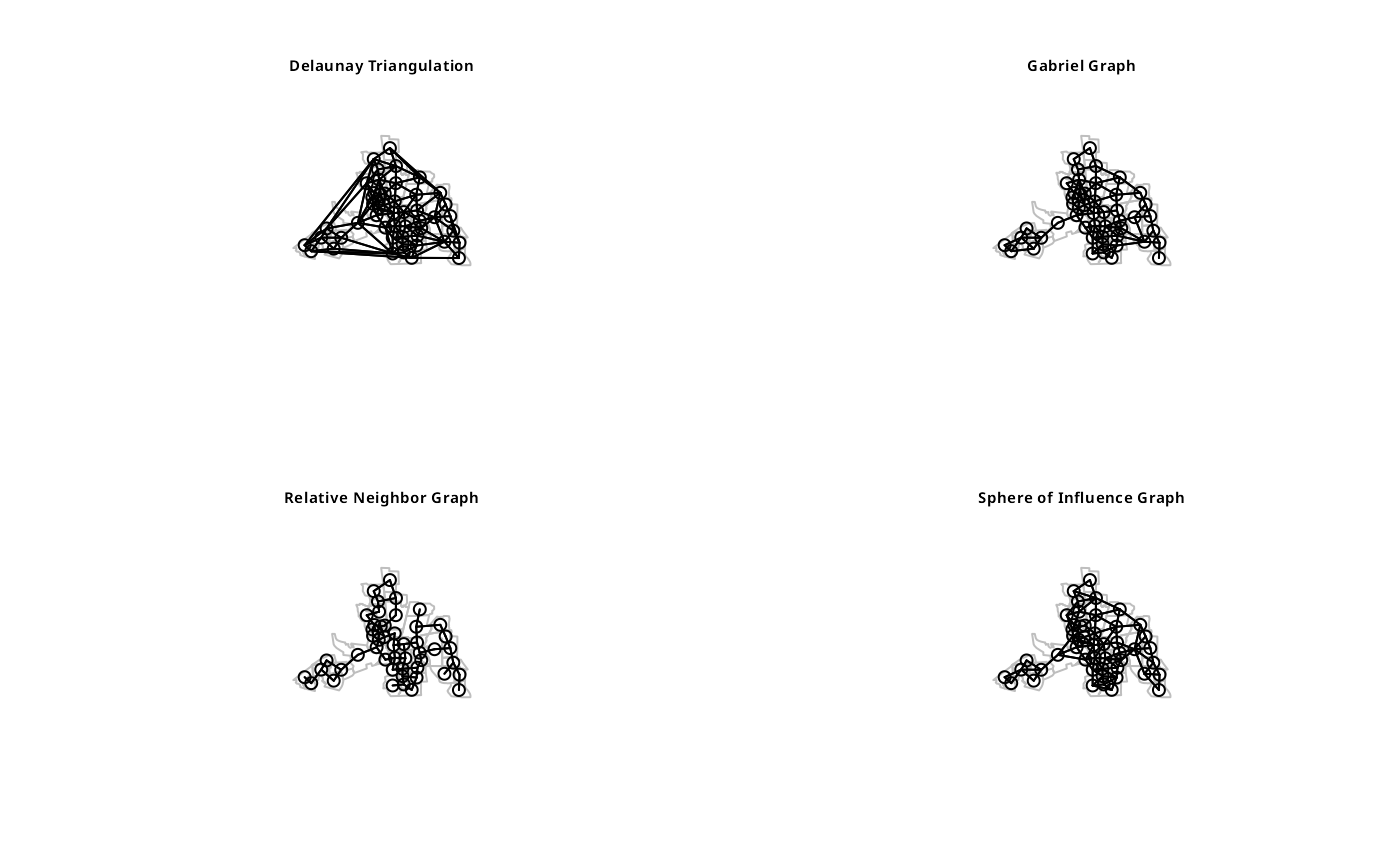
par(mfrow=c(2,2))
plot(st_geometry(columbus), border="grey")
plot(col.tri.nb,coords,add=TRUE)
title(main="Delaunay Triangulation", cex.main=0.6)
plot(st_geometry(columbus), border="grey")
plot(col.gab.nb, coords, add=TRUE)
title(main="Gabriel Graph", cex.main=0.6)
plot(st_geometry(columbus), border="grey")
plot(col.rel.nb, coords, add=TRUE)
title(main="Relative Neighbor Graph", cex.main=0.6)
plot(st_geometry(columbus), border="grey")
if (require("dbscan", quietly=TRUE)) {
  col.soi.nb <- graph2nb(soi.graph(col.tri.nb,coords), sym=TRUE)
  plot(col.soi.nb, coords, add=TRUE)
  title(main="Sphere of Influence Graph", cex.main=0.6)
}
#> 
#> Attaching package: ‘dbscan’
#> The following object is masked from ‘package:stats’:
#> 
#>     as.dendrogram

par(mfrow=c(1,1))
col.tri.nb_sf <- tri2nb(sf_obj)
all.equal(col.tri.nb, col.tri.nb_sf, check.attributes=FALSE)
#> [1] TRUE
col.tri.nb_sp <- tri2nb(sp_obj)
all.equal(col.tri.nb, col.tri.nb_sp, check.attributes=FALSE)
#> [1] TRUE
if (require("dbscan", quietly=TRUE)) {
  col.soi.nb_sf <- graph2nb(soi.graph(col.tri.nb, sf_obj), sym=TRUE)
  all.equal(col.soi.nb, col.soi.nb_sf, check.attributes=FALSE)
  col.soi.nb_sp <- graph2nb(soi.graph(col.tri.nb, sp_obj), sym=TRUE)
  all.equal(col.soi.nb, col.soi.nb_sp, check.attributes=FALSE)
}
#> [1] TRUE
col.gab.nb_sp <- graph2nb(gabrielneigh(sp_obj), sym=TRUE)
all.equal(col.gab.nb, col.gab.nb_sp, check.attributes=FALSE)
#> [1] TRUE
col.gab.nb_sf <- graph2nb(gabrielneigh(sf_obj), sym=TRUE)
all.equal(col.gab.nb, col.gab.nb_sf, check.attributes=FALSE)
#> [1] TRUE
col.rel.nb_sp <- graph2nb(relativeneigh(sp_obj), sym=TRUE)
all.equal(col.rel.nb, col.rel.nb_sp, check.attributes=FALSE)
#> [1] TRUE
col.rel.nb_sf <- graph2nb(relativeneigh(sf_obj), sym=TRUE)
all.equal(col.rel.nb, col.rel.nb_sf, check.attributes=FALSE)
#> [1] TRUE
dx <- rep(0.25*0:4,5)
dy <- c(rep(0,5),rep(0.25,5),rep(0.5,5), rep(0.75,5),rep(1,5))
m <- cbind(c(dx, dx, 3+dx, 3+dx), c(dy, 3+dy, dy, 3+dy))
cat(try(res <- gabrielneigh(m), silent=TRUE), "\n")
#> Error in gabrielneigh(m) : number of neighbours overrun - increase nnmult
#>  
res <- gabrielneigh(m, nnmult=4)
summary(graph2nb(res))
#> Neighbour list object:
#> Number of regions: 100 
#> Number of nonzero links: 342 
#> Percentage nonzero weights: 3.42 
#> Average number of links: 3.42 
#> 1 region with no links:
#> 100
#> Non-symmetric neighbours list
#> Link number distribution:
#> 
#>  0  1  2  3  4  5 
#>  1  8 10 18 55  8 
#> 8 least connected regions:
#> 46 47 48 49 96 97 98 99 with 1 link
#> 8 most connected regions:
#> 10 15 20 25 30 35 40 45 with 5 links
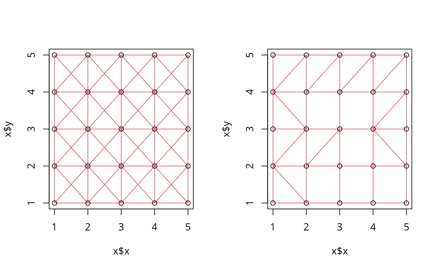
grd <- as.matrix(expand.grid(x=1:5, y=1:5)) #gridded data
r2 <- gabrielneigh(grd)
set.seed(1)
grd1 <- as.matrix(expand.grid(x=1:5, y=1:5)) + matrix(runif(50, .0001, .0006), nrow=25)
r3 <- gabrielneigh(grd1)
opar <- par(mfrow=c(1,2))
plot(r2, show=TRUE, linecol=2)
plot(r3, show=TRUE, linecol=2)

par(opar)
# example of reading points with readr::read_csv() yielding a tibble
load(system.file("etc/misc/coords.rda", package="spdep"))
class(coords)
#> [1] "spec_tbl_df" "tbl_df"      "tbl"         "data.frame" 
graph2nb(gabrielneigh(coords))
#> Neighbour list object:
#> Number of regions: 100 
#> Number of nonzero links: 179 
#> Percentage nonzero weights: 1.79 
#> Average number of links: 1.79 
#> 23 regions with no links:
#> 22 39 43 53 58 61 66 70 71 73 76 78 81 88 90 93 94 95 96 97 98 99 100
#> Non-symmetric neighbours list
graph2nb(relativeneigh(coords))
#> Neighbour list object:
#> Number of regions: 100 
#> Number of nonzero links: 117 
#> Percentage nonzero weights: 1.17 
#> Average number of links: 1.17 
#> 31 regions with no links:
#> 22 29 33 39 41 42 43 44 53 58 61 64 65 66 70 71 73 75 76 78 81 88 90 93
#> 94 95 96 97 98 99 100
#> Non-symmetric neighbours list