spatial join, spatial filter

Usage

st_join(x, y, join, ...)

# S3 method for class 'sf'
st_join(
  x,
  y,
  join = st_intersects,
  ...,
  suffix = c(".x", ".y"),
  left = TRUE,
  largest = FALSE
)

st_filter(x, y, ...)

# S3 method for class 'sf'
st_filter(x, y, ..., .predicate = st_intersects)

Arguments

x: object of class sf
y: object of class sf
join: geometry predicate function with the same profile as st_intersects; see details
...: for st_join: arguments passed on to the join function or to st_intersection when largest is TRUE; for st_filter arguments passed on to the .predicate function, e.g. prepared, or a pattern for st_relate
suffix: length 2 character vector; see merge
left: logical; if TRUE return the left join, otherwise an inner join; see details. see also left_join
largest: logical; if TRUE, return x features augmented with the fields of y that have the largest overlap with each of the features of x; see https://github.com/r-spatial/sf/issues/578
.predicate: geometry predicate function with the same profile as st_intersects; see details

Value

an object of class sf, joined based on geometry

Details

alternative values for argument join are:

st_contains_properly,
st_contains,
st_covered_by,
st_covers,
st_crosses,
st_disjoint,
st_equals_exact,
st_equals,
st_is_within_distance,
st_nearest_feature,
st_overlaps,
st_touches,
st_within,
st_relate (which will require pattern to be set),
or any user-defined function of the same profile as the above

A left join returns all records of the x object with y fields for non-matched records filled with NA values; an inner join returns only records that spatially match.

To replicate the results of st_within(x, y) you will need to use st_join(x, y, join = "st_within", left = FALSE).

Examples

a = st_sf(a = 1:3,
 geom = st_sfc(st_point(c(1,1)), st_point(c(2,2)), st_point(c(3,3))))
b = st_sf(a = 11:14,
 geom = st_sfc(st_point(c(10,10)), st_point(c(2,2)), st_point(c(2,2)), st_point(c(3,3))))
st_join(a, b)
#> Simple feature collection with 4 features and 2 fields
#> Geometry type: POINT
#> Dimension:     XY
#> Bounding box:  xmin: 1 ymin: 1 xmax: 3 ymax: 3
#> CRS:           NA
#>     a.x a.y        geom
#> 1     1  NA POINT (1 1)
#> 2     2  12 POINT (2 2)
#> 2.1   2  13 POINT (2 2)
#> 3     3  14 POINT (3 3)
st_join(a, b, left = FALSE)
#> Simple feature collection with 3 features and 2 fields
#> Geometry type: POINT
#> Dimension:     XY
#> Bounding box:  xmin: 2 ymin: 2 xmax: 3 ymax: 3
#> CRS:           NA
#>     a.x a.y        geom
#> 2     2  12 POINT (2 2)
#> 2.1   2  13 POINT (2 2)
#> 3     3  14 POINT (3 3)
# two ways to aggregate y's attribute values outcome over x's geometries:
st_join(a, b) %>% aggregate(list(.$a.x), mean)
#> Simple feature collection with 3 features and 3 fields
#> Attribute-geometry relationships: aggregate (2), identity (1)
#> Geometry type: POINT
#> Dimension:     XY
#> Bounding box:  xmin: 1 ymin: 1 xmax: 3 ymax: 3
#> CRS:           NA
#>   Group.1 a.x  a.y    geometry
#> 1       1   1   NA POINT (1 1)
#> 2       2   2 12.5 POINT (2 2)
#> 3       3   3 14.0 POINT (3 3)
if (require(dplyr, quietly = TRUE)) {
 st_join(a, b) %>% group_by(a.x) %>% summarise(mean(a.y))
}
#> Simple feature collection with 3 features and 2 fields
#> Geometry type: POINT
#> Dimension:     XY
#> Bounding box:  xmin: 1 ymin: 1 xmax: 3 ymax: 3
#> CRS:           NA
#> # A tibble: 3 × 3
#>     a.x `mean(a.y)`    geom
#>   <int>       <dbl> <POINT>
#> 1     1        NA     (1 1)
#> 2     2        12.5   (2 2)
#> 3     3        14     (3 3)
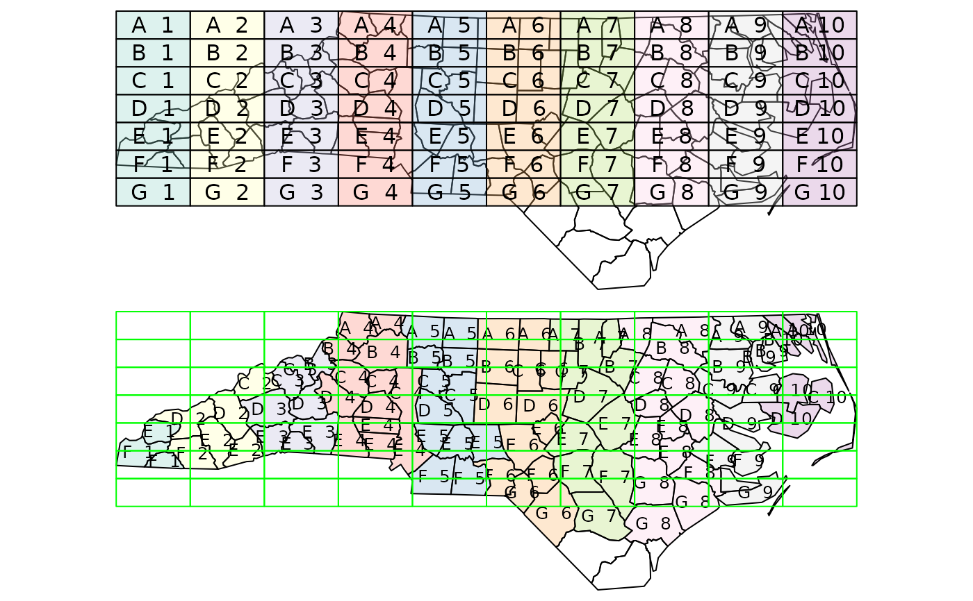
# example of largest = TRUE:
nc <- st_transform(st_read(system.file("shape/nc.shp", package="sf")), 2264)                
#> Reading layer `nc' from data source 
#>   `/home/runner/work/_temp/Library/sf/shape/nc.shp' using driver `ESRI Shapefile'
#> Simple feature collection with 100 features and 14 fields
#> Geometry type: MULTIPOLYGON
#> Dimension:     XY
#> Bounding box:  xmin: -84.32385 ymin: 33.88199 xmax: -75.45698 ymax: 36.58965
#> Geodetic CRS:  NAD27
gr = st_sf(
    label = apply(expand.grid(1:10, LETTERS[10:1])[,2:1], 1, paste0, collapse = " "),
    geom = st_make_grid(st_as_sfc(st_bbox(nc))))
gr$col = sf.colors(10, categorical = TRUE, alpha = .3)
# cut, to check, NA's work out:
gr = gr[-(1:30),]
nc_j <- st_join(nc, gr, largest = TRUE)
#> Warning: attribute variables are assumed to be spatially constant throughout all geometries
# the two datasets:
opar = par(mfrow = c(2,1), mar = rep(0,4))
plot(st_geometry(nc_j))
plot(st_geometry(gr), add = TRUE, col = gr$col)
text(st_coordinates(st_centroid(gr)), labels = gr$label)
#> Warning: st_centroid assumes attributes are constant over geometries
# the joined dataset:
plot(st_geometry(nc_j), border = 'black', col = nc_j$col)
text(st_coordinates(st_centroid(nc_j)), labels = nc_j$label, cex = .8)
#> Warning: st_centroid assumes attributes are constant over geometries
plot(st_geometry(gr), border = 'green', add = TRUE)

par(opar)
# st_filter keeps the geometries in x where .predicate(x,y) returns any match in y for x
st_filter(a, b)
#> Simple feature collection with 2 features and 1 field
#> Geometry type: POINT
#> Dimension:     XY
#> Bounding box:  xmin: 2 ymin: 2 xmax: 3 ymax: 3
#> CRS:           NA
#>   a        geom
#> 1 2 POINT (2 2)
#> 2 3 POINT (3 3)
# for an anti-join, use the union of y
st_filter(a, st_union(b), .predicate = st_disjoint)
#> Simple feature collection with 1 feature and 1 field
#> Geometry type: POINT
#> Dimension:     XY
#> Bounding box:  xmin: 1 ymin: 1 xmax: 1 ymax: 1
#> CRS:           NA
#>   a        geom
#> 1 1 POINT (1 1)