Tidyverse methods for sf objects. Geometries are sticky, use as.data.frame to let dplyr's own methods drop them.
Use these methods after loading the tidyverse package with the generic (or after loading package tidyverse).
Usage
filter.sf(.data, ..., .dots)

arrange.sf(.data, ..., .dots)

group_by.sf(.data, ..., add = FALSE)

ungroup.sf(x, ...)

rowwise.sf(x, ...)

mutate.sf(.data, ..., .dots)

transmute.sf(.data, ..., .dots)

select.sf(.data, ...)

rename.sf(.data, ...)

rename_with.sf(.data, .fn, .cols, ...)

slice.sf(.data, ..., .dots)

summarise.sf(.data, ..., .dots, do_union = TRUE, is_coverage = FALSE)

count.sf(x, ..., wt = NULL, sort = FALSE, name = "n", .drop_geometry = FALSE)

distinct.sf(.data, ..., .keep_all = FALSE, exact = FALSE, par = 0)

gather.sf(
  data,
  key,
  value,
  ...,
  na.rm = FALSE,
  convert = FALSE,
  factor_key = FALSE
)

pivot_longer.sf(
  data,
  cols,
  names_to = "name",
  names_prefix = NULL,
  names_sep = NULL,
  names_pattern = NULL,
  names_ptypes = NULL,
  names_transform = NULL,
  names_repair = "check_unique",
  values_to = "value",
  values_drop_na = FALSE,
  values_ptypes = NULL,
  values_transform = NULL,
  ...
)

pivot_wider.sf(
  data,
  ...,
  id_cols = NULL,
  id_expand = FALSE,
  names_from = name,
  names_prefix = "",
  names_sep = "_",
  names_glue = NULL,
  names_sort = FALSE,
  names_vary = "fastest",
  names_expand = FALSE,
  names_repair = "check_unique",
  values_from = value,
  values_fill = NULL,
  values_fn = NULL,
  unused_fn = NULL
)

spread.sf(
  data,
  key,
  value,
  fill = NA,
  convert = FALSE,
  drop = TRUE,
  sep = NULL
)

sample_n.sf(tbl, size, replace = FALSE, weight = NULL, .env = parent.frame())

sample_frac.sf(
  tbl,
  size = 1,
  replace = FALSE,
  weight = NULL,
  .env = parent.frame()
)

group_split.sf(.tbl, ..., .keep = TRUE)

nest.sf(.data, ...)

separate.sf(
  data,
  col,
  into,
  sep = "[^[:alnum:]]+",
  remove = TRUE,
  convert = FALSE,
  extra = "warn",
  fill = "warn",
  ...
)

separate_rows.sf(data, ..., sep = "[^[:alnum:]]+", convert = FALSE)

unite.sf(data, col, ..., sep = "_", remove = TRUE)

unnest.sf(data, ..., .preserve = NULL)

drop_na.sf(x, ...)

inner_join.sf(x, y, by = NULL, copy = FALSE, suffix = c(".x", ".y"), ...)

left_join.sf(x, y, by = NULL, copy = FALSE, suffix = c(".x", ".y"), ...)

right_join.sf(x, y, by = NULL, copy = FALSE, suffix = c(".x", ".y"), ...)

full_join.sf(x, y, by = NULL, copy = FALSE, suffix = c(".x", ".y"), ...)

semi_join.sf(x, y, by = NULL, copy = FALSE, suffix = c(".x", ".y"), ...)

anti_join.sf(x, y, by = NULL, copy = FALSE, suffix = c(".x", ".y"), ...)
Arguments
- .data
data object of class sf
- ...
other arguments
- .dots
see corresponding function in package
dplyr- add
see corresponding function in dplyr
- x, y
A pair of data frames, data frame extensions (e.g. a tibble), or lazy data frames (e.g. from dbplyr or dtplyr). See Methods, below, for more details.
- .fn, .cols
see original docs
- do_union
logical; in case
summarydoes not create a geometry column, should geometries be created by unioning using st_union, or simply by combining using st_combine? Using st_union resolves internal boundaries, but in case of unioning points, this will likely change the order of the points; see Details.- is_coverage
logical; if
do_unionisTRUE, use an optimized algorithm for features that form a polygonal coverage (have no overlaps)- wt
see original function docs
- sort
see original function docs
- name
see original function docs
- .drop_geometry
logical; if
TRUE, remove geometry column before computing counts- .keep_all
see corresponding function in dplyr
- exact
logical; if
TRUEuse st_equals_exact for geometry comparisons- par
numeric; passed on to st_equals_exact
- data
see original function docs
- key
see original function docs
- value
see original function docs
- na.rm
see original function docs
- convert
see separate_rows
- factor_key
see original function docs
- cols
see original function docs
- names_to, names_pattern, names_ptypes, names_transform
- names_prefix, names_sep, names_repair
see original function docs.
- values_to, values_drop_na, values_ptypes, values_transform
- id_cols, id_expand, names_from, names_sort, names_glue, names_vary, names_expand
- values_from, values_fill, values_fn, unused_fn
- fill
see original function docs
- drop
see original function docs
- sep
see separate_rows
- tbl
see original function docs
- size
see original function docs
- replace
see original function docs
- weight
see original function docs
- .env
see original function docs
- .tbl
see original function docs
- .keep
see original function docs
- col
see separate
- into
see separate
- remove
see separate
- extra
see separate
- .preserve
see unnest
- by
A join specification created with
join_by(), or a character vector of variables to join by.If
NULL, the default,*_join()will perform a natural join, using all variables in common acrossxandy. A message lists the variables so that you can check they're correct; suppress the message by supplyingbyexplicitly.To join on different variables between
xandy, use ajoin_by()specification. For example,join_by(a == b)will matchx$atoy$b.To join by multiple variables, use a
join_by()specification with multiple expressions. For example,join_by(a == b, c == d)will matchx$atoy$bandx$ctoy$d. If the column names are the same betweenxandy, you can shorten this by listing only the variable names, likejoin_by(a, c).join_by()can also be used to perform inequality, rolling, and overlap joins. See the documentation at ?join_by for details on these types of joins.For simple equality joins, you can alternatively specify a character vector of variable names to join by. For example,
by = c("a", "b")joinsx$atoy$aandx$btoy$b. If variable names differ betweenxandy, use a named character vector likeby = c("x_a" = "y_a", "x_b" = "y_b").To perform a cross-join, generating all combinations of
xandy, seecross_join().- copy
If
xandyare not from the same data source, andcopyisTRUE, thenywill be copied into the same src asx. This allows you to join tables across srcs, but it is a potentially expensive operation so you must opt into it.- suffix
If there are non-joined duplicate variables in
xandy, these suffixes will be added to the output to disambiguate them. Should be a character vector of length 2.
Value
an object of class sf
Details
select keeps the geometry regardless whether it is selected or not; to deselect it, first pipe through as.data.frame to let dplyr's own select drop it.
In case one or more of the arguments (expressions) in the summarise call creates a geometry list-column, the first of these will be the (active) geometry of the returned object. If this is not the case, a geometry column is created, depending on the value of do_union.
In case do_union is FALSE, summarise will simply combine geometries using c.sfg. When polygons sharing a boundary are combined, this leads to geometries that are invalid; see for instance https://github.com/r-spatial/sf/issues/681.
The functions count and tally drop all geometries.
For counting geometries use summarise(.data, n = n(), .by = "geometry").
distinct gives distinct records for which all attributes and geometries are distinct; st_equals is used to find out which geometries are distinct.
nest assumes that a simple feature geometry list-column was among the columns that were nested.
Examples
if (require(dplyr, quietly = TRUE)) {
nc = read_sf(system.file("shape/nc.shp", package="sf"))
nc |> filter(AREA > .1) |> plot()
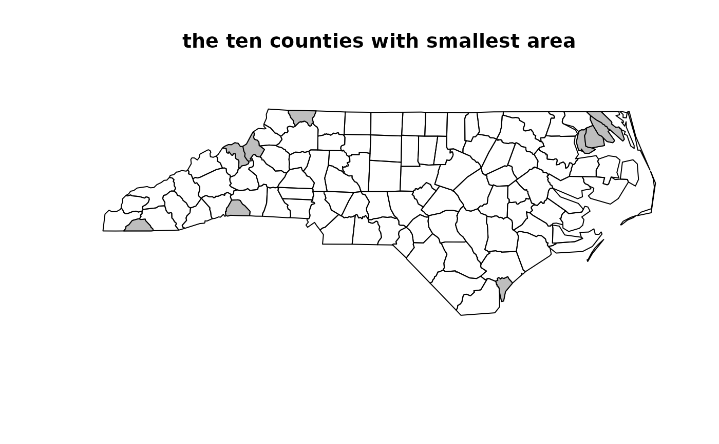
# plot 10 smallest counties in grey:
st_geometry(nc) |> plot()
nc |> select(AREA) |> arrange(AREA) |> slice(1:10) |> plot(add = TRUE, col = 'grey')
title("the ten counties with smallest area")
nc2 <- nc |> mutate(area10 = AREA/10)
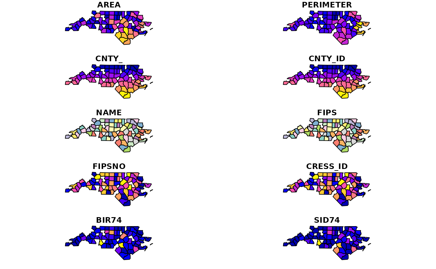
nc |> slice(1:2)
}
#> Warning: plotting the first 10 out of 14 attributes; use max.plot = 14 to plot all
 #> Simple feature collection with 2 features and 14 fields
#> Geometry type: MULTIPOLYGON
#> Dimension: XY
#> Bounding box: xmin: -81.74107 ymin: 36.23436 xmax: -80.90344 ymax: 36.58965
#> Geodetic CRS: NAD27
#> # A tibble: 2 × 15
#> AREA PERIMETER CNTY_ CNTY_ID NAME FIPS FIPSNO CRESS_ID BIR74 SID74 NWBIR74
#> <dbl> <dbl> <dbl> <dbl> <chr> <chr> <dbl> <int> <dbl> <dbl> <dbl>
#> 1 0.114 1.44 1825 1825 Ashe 37009 37009 5 1091 1 10
#> 2 0.061 1.23 1827 1827 Alleg… 37005 37005 3 487 0 10
#> # ℹ 4 more variables: BIR79 <dbl>, SID79 <dbl>, NWBIR79 <dbl>,
#> # geometry <MULTIPOLYGON [°]>
# plot 10 smallest counties in grey:
if (require(dplyr, quietly = TRUE)) {
st_geometry(nc) |> plot()
nc |> select(AREA) |> arrange(AREA) |> slice(1:10) |> plot(add = TRUE, col = 'grey')
title("the ten counties with smallest area")
}
if (require(dplyr, quietly = TRUE)) {
nc$area_cl = cut(nc$AREA, c(0, .1, .12, .15, .25))
nc |> group_by(area_cl) |> class()
}
#> [1] "sf" "grouped_df" "tbl_df" "tbl" "data.frame"
if (require(dplyr, quietly = TRUE)) {
nc2 <- nc |> mutate(area10 = AREA/10)
}
if (require(dplyr, quietly = TRUE)) {
nc |> transmute(AREA = AREA/10) |> class()
}
#> [1] "sf" "tbl_df" "tbl" "data.frame"
if (require(dplyr, quietly = TRUE)) {
nc |> select(SID74, SID79) |> names()
nc |> select(SID74, SID79) |> class()
}
#> [1] "sf" "tbl_df" "tbl" "data.frame"
if (require(dplyr, quietly = TRUE)) {
nc2 <- nc |> rename(area = AREA)
}
if (require(dplyr, quietly = TRUE)) {
nc |> slice(1:2)
}
#> Simple feature collection with 2 features and 15 fields
#> Geometry type: MULTIPOLYGON
#> Dimension: XY
#> Bounding box: xmin: -81.74107 ymin: 36.23436 xmax: -80.90344 ymax: 36.58965
#> Geodetic CRS: NAD27
#> # A tibble: 2 × 16
#> AREA PERIMETER CNTY_ CNTY_ID NAME FIPS FIPSNO CRESS_ID BIR74 SID74 NWBIR74
#> <dbl> <dbl> <dbl> <dbl> <chr> <chr> <dbl> <int> <dbl> <dbl> <dbl>
#> 1 0.114 1.44 1825 1825 Ashe 37009 37009 5 1091 1 10
#> 2 0.061 1.23 1827 1827 Alleg… 37005 37005 3 487 0 10
#> # ℹ 5 more variables: BIR79 <dbl>, SID79 <dbl>, NWBIR79 <dbl>,
#> # geometry <MULTIPOLYGON [°]>, area_cl <fct>
if (require(dplyr, quietly = TRUE)) {
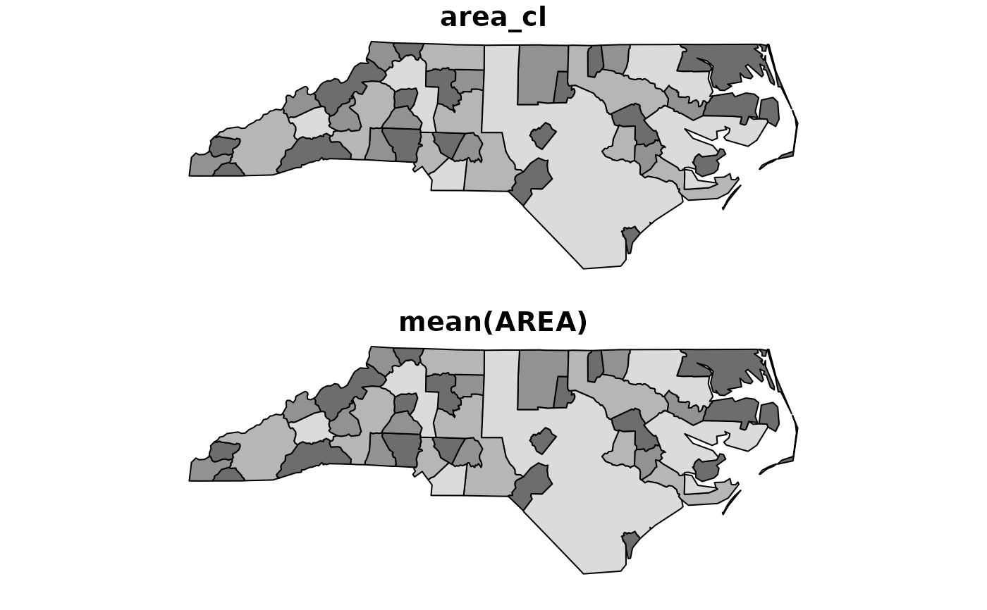
nc$area_cl = cut(nc$AREA, c(0, .1, .12, .15, .25))
nc.g <- nc |> group_by(area_cl)
nc.g |> summarise(mean(AREA))
nc.g |> summarise(mean(AREA)) |> plot(col = grey(3:6 / 7))
nc |> as.data.frame() |> summarise(mean(AREA))
# counting geometries (after duplicating each row):
nc.dupl <- nc[rep(seq_along(nc), each = 2), ]
nc.dupl |> summarise(n = n(), .by = "geometry")
}
#> Simple feature collection with 2 features and 14 fields
#> Geometry type: MULTIPOLYGON
#> Dimension: XY
#> Bounding box: xmin: -81.74107 ymin: 36.23436 xmax: -80.90344 ymax: 36.58965
#> Geodetic CRS: NAD27
#> # A tibble: 2 × 15
#> AREA PERIMETER CNTY_ CNTY_ID NAME FIPS FIPSNO CRESS_ID BIR74 SID74 NWBIR74
#> <dbl> <dbl> <dbl> <dbl> <chr> <chr> <dbl> <int> <dbl> <dbl> <dbl>
#> 1 0.114 1.44 1825 1825 Ashe 37009 37009 5 1091 1 10
#> 2 0.061 1.23 1827 1827 Alleg… 37005 37005 3 487 0 10
#> # ℹ 4 more variables: BIR79 <dbl>, SID79 <dbl>, NWBIR79 <dbl>,
#> # geometry <MULTIPOLYGON [°]>
# plot 10 smallest counties in grey:
if (require(dplyr, quietly = TRUE)) {
st_geometry(nc) |> plot()
nc |> select(AREA) |> arrange(AREA) |> slice(1:10) |> plot(add = TRUE, col = 'grey')
title("the ten counties with smallest area")
}
if (require(dplyr, quietly = TRUE)) {
nc$area_cl = cut(nc$AREA, c(0, .1, .12, .15, .25))
nc |> group_by(area_cl) |> class()
}
#> [1] "sf" "grouped_df" "tbl_df" "tbl" "data.frame"
if (require(dplyr, quietly = TRUE)) {
nc2 <- nc |> mutate(area10 = AREA/10)
}
if (require(dplyr, quietly = TRUE)) {
nc |> transmute(AREA = AREA/10) |> class()
}
#> [1] "sf" "tbl_df" "tbl" "data.frame"
if (require(dplyr, quietly = TRUE)) {
nc |> select(SID74, SID79) |> names()
nc |> select(SID74, SID79) |> class()
}
#> [1] "sf" "tbl_df" "tbl" "data.frame"
if (require(dplyr, quietly = TRUE)) {
nc2 <- nc |> rename(area = AREA)
}
if (require(dplyr, quietly = TRUE)) {
nc |> slice(1:2)
}
#> Simple feature collection with 2 features and 15 fields
#> Geometry type: MULTIPOLYGON
#> Dimension: XY
#> Bounding box: xmin: -81.74107 ymin: 36.23436 xmax: -80.90344 ymax: 36.58965
#> Geodetic CRS: NAD27
#> # A tibble: 2 × 16
#> AREA PERIMETER CNTY_ CNTY_ID NAME FIPS FIPSNO CRESS_ID BIR74 SID74 NWBIR74
#> <dbl> <dbl> <dbl> <dbl> <chr> <chr> <dbl> <int> <dbl> <dbl> <dbl>
#> 1 0.114 1.44 1825 1825 Ashe 37009 37009 5 1091 1 10
#> 2 0.061 1.23 1827 1827 Alleg… 37005 37005 3 487 0 10
#> # ℹ 5 more variables: BIR79 <dbl>, SID79 <dbl>, NWBIR79 <dbl>,
#> # geometry <MULTIPOLYGON [°]>, area_cl <fct>
if (require(dplyr, quietly = TRUE)) {
nc$area_cl = cut(nc$AREA, c(0, .1, .12, .15, .25))
nc.g <- nc |> group_by(area_cl)
nc.g |> summarise(mean(AREA))
nc.g |> summarise(mean(AREA)) |> plot(col = grey(3:6 / 7))
nc |> as.data.frame() |> summarise(mean(AREA))
# counting geometries (after duplicating each row):
nc.dupl <- nc[rep(seq_along(nc), each = 2), ]
nc.dupl |> summarise(n = n(), .by = "geometry")
}
 #> Simple feature collection with 16 features and 1 field
#> Geometry type: MULTIPOLYGON
#> Dimension: XY
#> Bounding box: xmin: -81.74107 ymin: 35.99472 xmax: -75.77316 ymax: 36.58965
#> Geodetic CRS: NAD27
#> # A tibble: 16 × 2
#> geometry n
#> <MULTIPOLYGON [°]> <int>
#> 1 (((-81.47276 36.23436, -81.54084 36.27251, -81.56198 36.27359, -81.633… 2
#> 2 (((-81.23989 36.36536, -81.24069 36.37942, -81.26284 36.40504, -81.266… 2
#> 3 (((-80.45634 36.24256, -80.47639 36.25473, -80.53688 36.25674, -80.545… 2
#> 4 (((-76.00897 36.3196, -76.01735 36.33773, -76.03288 36.33598, -76.0439… 2
#> 5 (((-77.21767 36.24098, -77.23461 36.2146, -77.29861 36.21153, -77.2935… 2
#> 6 (((-76.74506 36.23392, -76.98069 36.23024, -76.99475 36.23558, -77.130… 2
#> 7 (((-76.00897 36.3196, -75.95718 36.19377, -75.98134 36.16973, -76.1831… 2
#> 8 (((-76.56251 36.34057, -76.60424 36.31498, -76.64822 36.31532, -76.688… 2
#> 9 (((-78.30876 36.26004, -78.28293 36.29188, -78.32125 36.54553, -78.051… 2
#> 10 (((-80.02567 36.25023, -80.45301 36.25709, -80.43531 36.55104, -80.048… 2
#> 11 (((-79.53051 36.24614, -79.5103 36.54766, -79.21706 36.54978, -79.1443… 2
#> 12 (((-79.53051 36.24614, -79.53058 36.23616, -80.02567 36.25023, -80.024… 2
#> 13 (((-78.74912 36.06359, -78.78841 36.06218, -78.80405 36.08094, -78.810… 2
#> 14 (((-78.8068 36.23158, -78.95108 36.23384, -79.15927 36.23367, -79.1443… 2
#> 15 (((-78.49252 36.17359, -78.51472 36.17522, -78.51709 36.46148, -78.502… 2
#> 16 (((-77.33221 36.06798, -77.40531 35.99472, -77.42574 35.99606, -77.438… 2
if (require(dplyr, quietly = TRUE)) {
nc$area_cl <- cut(nc$AREA, c(0, .1, .12, .15, .25))
nc |> count(area_cl, .drop_geometry = TRUE)
}
#> # A tibble: 4 × 3
#> area_cl .drop_geometry n
#> <fct> <lgl> <int>
#> 1 (0,0.1] TRUE 35
#> 2 (0.1,0.12] TRUE 15
#> 3 (0.12,0.15] TRUE 22
#> 4 (0.15,0.25] TRUE 28
if (require(dplyr, quietly = TRUE)) {
nc[c(1:100, 1:10), ] |> distinct() |> nrow()
}
#> [1] 100
if (require(tidyr, quietly = TRUE) && require(dplyr, quietly = TRUE) && "geometry" %in% names(nc)) {
nc |> select(SID74, SID79) |> gather("VAR", "SID", -geometry) |> summary()
}
#> geometry VAR SID
#> MULTIPOLYGON :200 Length :200 Min. : 0.000
#> epsg:4267 : 0 N.unique : 2 1st Qu.: 2.000
#> +proj=long...: 0 N.blank : 0 Median : 5.000
#> Min.nchar: 5 Mean : 7.515
#> Max.nchar: 5 3rd Qu.: 9.000
#> Max. :57.000
if (require(tidyr, quietly = TRUE) && require(dplyr, quietly = TRUE) && "geometry" %in% names(nc)) {
nc$row = 1:100 # needed for spread to work
nc |> select(SID74, SID79, geometry, row) |>
gather("VAR", "SID", -geometry, -row) |>
spread(VAR, SID) |> head()
}
#> Simple feature collection with 6 features and 3 fields
#> Geometry type: MULTIPOLYGON
#> Dimension: XY
#> Bounding box: xmin: -81.74107 ymin: 36.07282 xmax: -75.77316 ymax: 36.58965
#> Geodetic CRS: NAD27
#> # A tibble: 6 × 4
#> geometry row SID74 SID79
#> <MULTIPOLYGON [°]> <int> <dbl> <dbl>
#> 1 (((-81.47276 36.23436, -81.54084 36.27251, -81.56198 36.273… 1 1 0
#> 2 (((-81.23989 36.36536, -81.24069 36.37942, -81.26284 36.405… 2 0 3
#> 3 (((-80.45634 36.24256, -80.47639 36.25473, -80.53688 36.256… 3 5 6
#> 4 (((-76.00897 36.3196, -76.01735 36.33773, -76.03288 36.3359… 4 1 2
#> 5 (((-77.21767 36.24098, -77.23461 36.2146, -77.29861 36.2115… 5 9 3
#> 6 (((-76.74506 36.23392, -76.98069 36.23024, -76.99475 36.235… 6 7 5
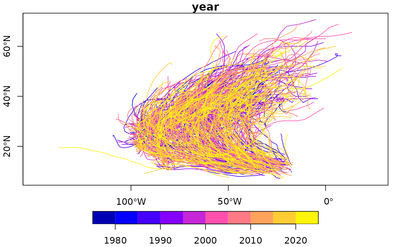
if (require(tidyr, quietly = TRUE) && require(dplyr, quietly = TRUE)) {
storms.sf = st_as_sf(storms, coords = c("long", "lat"), crs = 4326)
x <- storms.sf |> group_by(name, year) |> nest()
trs = lapply(x$data, function(tr) st_cast(st_combine(tr), "LINESTRING")[[1]]) |>
st_sfc(crs = 4326)
trs.sf = st_sf(x[,1:2], trs)
plot(trs.sf["year"], axes = TRUE)
}
#> Simple feature collection with 16 features and 1 field
#> Geometry type: MULTIPOLYGON
#> Dimension: XY
#> Bounding box: xmin: -81.74107 ymin: 35.99472 xmax: -75.77316 ymax: 36.58965
#> Geodetic CRS: NAD27
#> # A tibble: 16 × 2
#> geometry n
#> <MULTIPOLYGON [°]> <int>
#> 1 (((-81.47276 36.23436, -81.54084 36.27251, -81.56198 36.27359, -81.633… 2
#> 2 (((-81.23989 36.36536, -81.24069 36.37942, -81.26284 36.40504, -81.266… 2
#> 3 (((-80.45634 36.24256, -80.47639 36.25473, -80.53688 36.25674, -80.545… 2
#> 4 (((-76.00897 36.3196, -76.01735 36.33773, -76.03288 36.33598, -76.0439… 2
#> 5 (((-77.21767 36.24098, -77.23461 36.2146, -77.29861 36.21153, -77.2935… 2
#> 6 (((-76.74506 36.23392, -76.98069 36.23024, -76.99475 36.23558, -77.130… 2
#> 7 (((-76.00897 36.3196, -75.95718 36.19377, -75.98134 36.16973, -76.1831… 2
#> 8 (((-76.56251 36.34057, -76.60424 36.31498, -76.64822 36.31532, -76.688… 2
#> 9 (((-78.30876 36.26004, -78.28293 36.29188, -78.32125 36.54553, -78.051… 2
#> 10 (((-80.02567 36.25023, -80.45301 36.25709, -80.43531 36.55104, -80.048… 2
#> 11 (((-79.53051 36.24614, -79.5103 36.54766, -79.21706 36.54978, -79.1443… 2
#> 12 (((-79.53051 36.24614, -79.53058 36.23616, -80.02567 36.25023, -80.024… 2
#> 13 (((-78.74912 36.06359, -78.78841 36.06218, -78.80405 36.08094, -78.810… 2
#> 14 (((-78.8068 36.23158, -78.95108 36.23384, -79.15927 36.23367, -79.1443… 2
#> 15 (((-78.49252 36.17359, -78.51472 36.17522, -78.51709 36.46148, -78.502… 2
#> 16 (((-77.33221 36.06798, -77.40531 35.99472, -77.42574 35.99606, -77.438… 2
if (require(dplyr, quietly = TRUE)) {
nc$area_cl <- cut(nc$AREA, c(0, .1, .12, .15, .25))
nc |> count(area_cl, .drop_geometry = TRUE)
}
#> # A tibble: 4 × 3
#> area_cl .drop_geometry n
#> <fct> <lgl> <int>
#> 1 (0,0.1] TRUE 35
#> 2 (0.1,0.12] TRUE 15
#> 3 (0.12,0.15] TRUE 22
#> 4 (0.15,0.25] TRUE 28
if (require(dplyr, quietly = TRUE)) {
nc[c(1:100, 1:10), ] |> distinct() |> nrow()
}
#> [1] 100
if (require(tidyr, quietly = TRUE) && require(dplyr, quietly = TRUE) && "geometry" %in% names(nc)) {
nc |> select(SID74, SID79) |> gather("VAR", "SID", -geometry) |> summary()
}
#> geometry VAR SID
#> MULTIPOLYGON :200 Length :200 Min. : 0.000
#> epsg:4267 : 0 N.unique : 2 1st Qu.: 2.000
#> +proj=long...: 0 N.blank : 0 Median : 5.000
#> Min.nchar: 5 Mean : 7.515
#> Max.nchar: 5 3rd Qu.: 9.000
#> Max. :57.000
if (require(tidyr, quietly = TRUE) && require(dplyr, quietly = TRUE) && "geometry" %in% names(nc)) {
nc$row = 1:100 # needed for spread to work
nc |> select(SID74, SID79, geometry, row) |>
gather("VAR", "SID", -geometry, -row) |>
spread(VAR, SID) |> head()
}
#> Simple feature collection with 6 features and 3 fields
#> Geometry type: MULTIPOLYGON
#> Dimension: XY
#> Bounding box: xmin: -81.74107 ymin: 36.07282 xmax: -75.77316 ymax: 36.58965
#> Geodetic CRS: NAD27
#> # A tibble: 6 × 4
#> geometry row SID74 SID79
#> <MULTIPOLYGON [°]> <int> <dbl> <dbl>
#> 1 (((-81.47276 36.23436, -81.54084 36.27251, -81.56198 36.273… 1 1 0
#> 2 (((-81.23989 36.36536, -81.24069 36.37942, -81.26284 36.405… 2 0 3
#> 3 (((-80.45634 36.24256, -80.47639 36.25473, -80.53688 36.256… 3 5 6
#> 4 (((-76.00897 36.3196, -76.01735 36.33773, -76.03288 36.3359… 4 1 2
#> 5 (((-77.21767 36.24098, -77.23461 36.2146, -77.29861 36.2115… 5 9 3
#> 6 (((-76.74506 36.23392, -76.98069 36.23024, -76.99475 36.235… 6 7 5
if (require(tidyr, quietly = TRUE) && require(dplyr, quietly = TRUE)) {
storms.sf = st_as_sf(storms, coords = c("long", "lat"), crs = 4326)
x <- storms.sf |> group_by(name, year) |> nest()
trs = lapply(x$data, function(tr) st_cast(st_combine(tr), "LINESTRING")[[1]]) |>
st_sfc(crs = 4326)
trs.sf = st_sf(x[,1:2], trs)
plot(trs.sf["year"], axes = TRUE)
}