Block up neighbour list for location-less observations

The function blocks up a neighbour list for known spatial locations to create a new neighbour list for multiple location-less observations know to belong to the spatial locations, using the identification tags of the locations as the key.

Usage

nb2blocknb(nb=NULL, ID, row.names = NULL)

Arguments

nb

an object of class nb with a list of integer vectors containing neighbour region number ids; if null, an nb object with no neighbours is created the length of unique(as.character(ID))

ID

identification tags of the locations for the location-less observations;

sort(unique(as.character(ID))) must be identical to

sort(as.character(attr(nb, "region.id")));

same length as row.names if provided.

row.names

character vector of observation ids to be added to the neighbours list as attribute region.id, default seq(1, nrow(x)); same length as ID if provided.

Details

Assume that there is a list of unique locations, then a neighbour list can build for that, to create an input neighbour list. This needs to be "unfolded", so that observations belonging to each unique location are observation neighbours, and observations belonging to the location neighbours of the unique location in question are also observation neighbours, finally removing the observation itself (because it should not be its own neighbour). This scenario also arises when say only post codes are available, and some post codes contain multiple observations, where all that is known is that they belong to a specific post code, not where they are located within it (given that the post code locations are known).

Value

The function returns an object of class nb with a list of integer vectors containing neighbour observation number ids.

Author

Roger Bivand Roger.Bivand@nhh.no

Examples

# \dontrun{
data(boston, package="spData")
summary(as.vector(table(boston.c$TOWN)))
#>    Min. 1st Qu.  Median    Mean 3rd Qu.    Max. 
#>     1.0     2.0     4.0     5.5     7.0    30.0 
townaggr <- aggregate(boston.utm, list(town=boston.c$TOWN), mean)
block.rel <- graph2nb(relativeneigh(as.matrix(townaggr[,2:3])),
 as.character(townaggr[,1]), sym=TRUE)
block.rel
#> Neighbour list object:
#> Number of regions: 92 
#> Number of nonzero links: 240 
#> Percentage nonzero weights: 2.835539 
#> Average number of links: 2.608696 
print(is.symmetric.nb(block.rel))
#> [1] TRUE
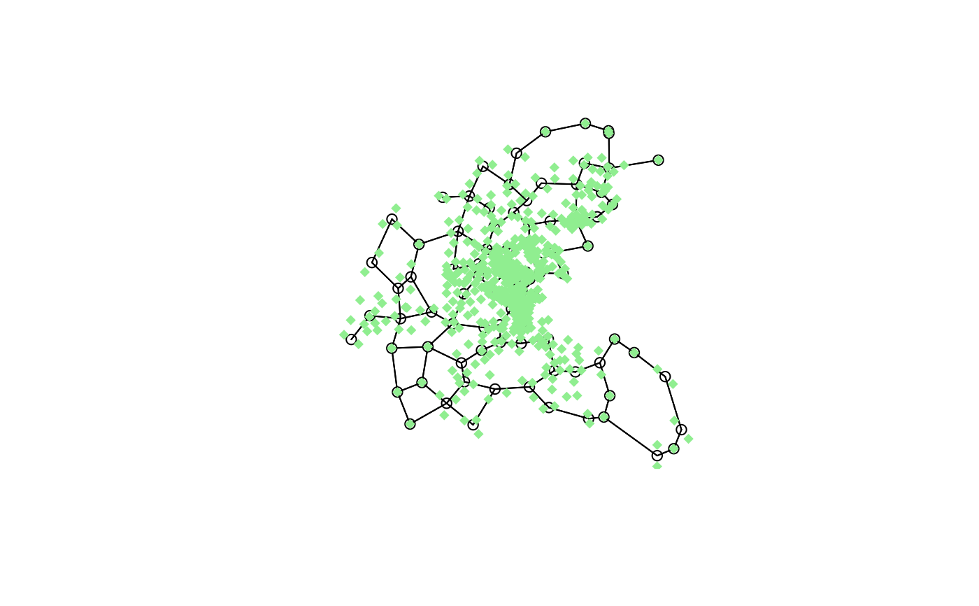
plot(block.rel, as.matrix(townaggr[,2:3]))
points(boston.utm, pch=18, col="lightgreen")

block.nb <- nb2blocknb(block.rel, as.character(boston.c$TOWN))
block.nb
#> Neighbour list object:
#> Number of regions: 506 
#> Number of nonzero links: 15234 
#> Percentage nonzero weights: 5.949945 
#> Average number of links: 30.10672 
print(is.symmetric.nb(block.nb))
#> [1] TRUE
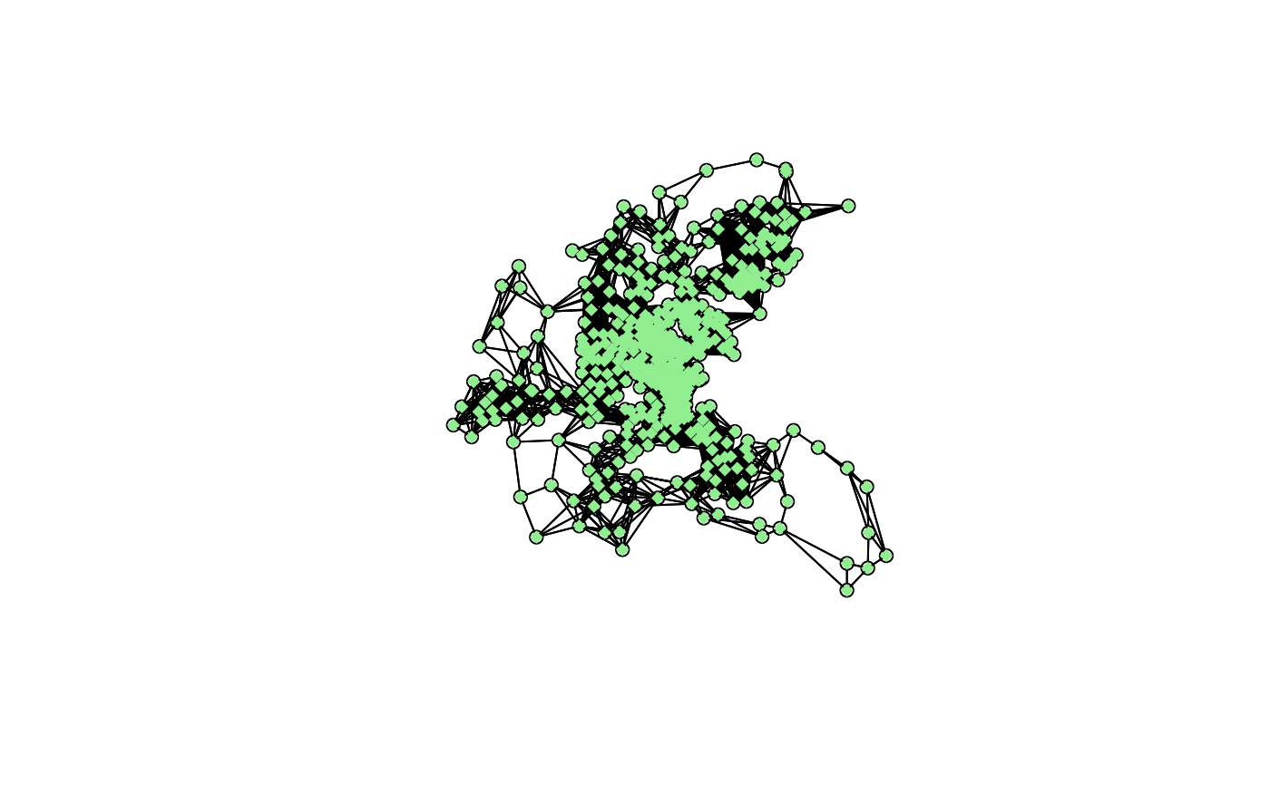
plot(block.nb, boston.utm)
points(boston.utm, pch=18, col="lightgreen")

n.comp.nb(block.nb)$nc
#> [1] 1
moran.test(boston.c$CMEDV, nb2listw(boston.soi))
#> 
#> 	Moran I test under randomisation
#> 
#> data:  boston.c$CMEDV  
#> weights: nb2listw(boston.soi)    
#> 
#> Moran I statistic standard deviate = 21.786, p-value < 2.2e-16
#> alternative hypothesis: greater
#> sample estimates:
#> Moran I statistic       Expectation          Variance 
#>       0.690285059      -0.001980198       0.001009685 
#> 
moran.test(boston.c$CMEDV, nb2listw(block.nb))
#> 
#> 	Moran I test under randomisation
#> 
#> data:  boston.c$CMEDV  
#> weights: nb2listw(block.nb)    
#> 
#> Moran I statistic standard deviate = 22.455, p-value < 2.2e-16
#> alternative hypothesis: greater
#> sample estimates:
#> Moran I statistic       Expectation          Variance 
#>      0.3122905961     -0.0019801980      0.0001958827 
#> 
block.nb <- nb2blocknb(NULL, as.character(boston.c$TOWN))
#> Warning: neighbour object has 92 sub-graphs
block.nb
#> Neighbour list object:
#> Number of regions: 506 
#> Number of nonzero links: 4868 
#> Percentage nonzero weights: 1.901295 
#> Average number of links: 9.620553 
#> 17 regions with no links:
#> 1, 55, 56, 57, 58, 65, 196, 257, 284, 285, 286, 287, 342, 343, 348,
#> 349, 354
#> 92 disjoint connected subgraphs
print(is.symmetric.nb(block.nb))
#> [1] TRUE
plot(block.nb, boston.utm)

n.comp.nb(block.nb)$nc
#> [1] 92
moran.test(boston.c$CMEDV, nb2listw(block.nb, zero.policy=TRUE), zero.policy=TRUE)
#> 
#> 	Moran I test under randomisation
#> 
#> data:  boston.c$CMEDV  
#> weights: nb2listw(block.nb, zero.policy = TRUE)  
#> n reduced by no-neighbour observations  
#> 
#> Moran I statistic standard deviate = 21.145, p-value < 2.2e-16
#> alternative hypothesis: greater
#> sample estimates:
#> Moran I statistic       Expectation          Variance 
#>      0.6188830566     -0.0020491803      0.0008623116 
#> 
# }